2.10 - The Binomial Distribution

Overview

A lot of random processes come down to counting successes: how many free throws go in, how many patients improve, how many students in a sample walk to school. When the setting meets four specific conditions, that count follows a binomial distribution, and you can find its probabilities, mean, and standard deviation with formulas instead of building a full table by hand. This topic covers how to recognize a binomial setting, calculate binomial probabilities, find and interpret the mean and standard deviation, and estimate binomial probabilities with a simulation.

What makes a random variable binomial

A binomial random variable

X

is a discrete random variable that counts the number of successes in

n

repeated independent trials, where each trial has only two possible outcomes (success or failure), the probability of success is

p

, and the probability of failure is

1 - p

To justify that a random variable is binomial, check all four conditions. The letters BINS help you remember them:

Binary: each trial has only two outcomes, success or failure. "Success" just means the outcome you're counting. It doesn't have to be a good thing.

Independent: the outcome of one trial doesn't change the probability of success on any other trial.

Number: the number of trials, $n$ , is fixed in advance.

Same probability: the probability of success, $p$ , is the same on every trial.

If all four hold, we say

X

has a binomial distribution with parameters

n

and

p

. On the AP exam, write it out in words, for example "

X

is binomial with

n = 20

and

p = 0.15

," and explain each condition in the context of the problem.

Sampling without replacement: the 10% condition

When you select people from a population without replacement, the trials aren't exactly independent. Picking one student who walks to school leaves slightly fewer walkers for the next pick. If the sample is small compared with the population, this change is too small to matter. The rule of thumb is the 10% condition: if the sample size is at most 10% of the population size (

n \le 0.10N

), you can treat the trials as independent. You'll use this condition all through Units 3 and 4.

Example 1: Binomial or not?

For each situation, decide whether

X

is a binomial random variable. Justify your answer.

(a) Roll a fair die 10 times.

X

= the number of 6s.

Binomial. Each roll is a 6 or not a 6 (binary). Rolls don't affect each other (independent). There are exactly

n = 10

rolls (number). The probability of a 6 is

p = \frac{1}{6}

on every roll (same probability).

(b) Draw cards from a shuffled standard deck until you get an ace.

X

= the number of cards drawn.

Not binomial. The number of trials isn't fixed in advance. You keep drawing until an ace shows up.

X

= the number of hearts.

Not binomial. The cards aren't replaced, so the probability of a heart changes from card to card (the trials aren't independent and

p

isn't the same). Since 10 cards is more than 10% of the 52-card deck, the change is too big to ignore.

(d) Suppose 15% of the 1,800 students at a large high school walk to school. Randomly select 20 of these students.

X

= the number of selected students who walk to school.

Binomial (approximately). Each student walks to school or doesn't (binary). There are

n = 20

students (number), and each has probability

p = 0.15

of walking to school (same probability). The sample is taken without replacement, but

20 \le 0.10(1{,}800) = 180

, so the 10% condition is met and we can treat the selections as independent.

The binomial probability formula

X

is binomial with

n

trials and probability of success

p

, the probability of exactly

x

successes is

P(X = x) = \binom{n}{x} p^x (1-p)^{n-x}, \qquad x = 0, 1, 2, \ldots, n

This is called the binomial probability function, and it's on the formula sheet. Each piece has a job:

$p^x$ is the probability of the $x$ successes. Since the trials are independent, you multiply.

$(1-p)^{n-x}$ is the probability of the $n - x$ failures.

$\binom{n}{x}$ , read " $n$ choose $x$ ," counts the different orders the $x$ successes could appear in among the $n$ trials:

\binom{n}{x} = \frac{n!}{x!\,(n-x)!}

For example, with

n = 3

trials there are

\binom{3}{2} = 3

ways to get exactly 2 successes: SSF, SFS, and FSS. Each order has probability

p^2(1-p)

, so

P(X = 2) = 3p^2(1-p)

Probabilities for a range of values

Many questions ask about more than one value. Translate the words into an inequality carefully. For a count,

X < 4

and

X \le 4

are different events, because one includes 4 and the other doesn't.

Words	Event	How to get it
exactly 4	$X = 4$	`binompdf(n, p, 4)`
at most 4	$X \le 4$	`binomcdf(n, p, 4)`
fewer than 4	$X < 4$ , same as $X \le 3$	`binomcdf(n, p, 3)`
at least 4	$X \ge 4$	$1 - P(X \le 3)$
more than 4	$X > 4$ , same as $X \ge 5$	$1 - P(X \le 4)$

On the TI-84

Press 2nd, VARS (DISTR). binompdf(n, p, x) gives

P(X = x)

. binomcdf(n, p, x) gives the cumulative probability

P(X \le x)

. For "at least" questions, use the complement:

P(X \ge 4) = 1 - P(X \le 3)

What to write on the AP exam: calculator syntax by itself doesn't earn full credit. Name the distribution and its parameters, show the event with its boundary and direction, then give the answer. For example: "

X

is binomial with

n = 20

and

p = 0.15

P(X \ge 6) = 1 - P(X \le 5) = 0.0673

." This is the same habit as Topic 2.6: show the setup, then the answer.

Example 2: Students who walk to school

Use the setting from Example 1(d): 20 randomly selected students, each with probability 0.15 of walking to school.

X

is binomial with

n = 20

and

p = 0.15

(a) Find the probability that exactly 2 of the students walk to school. (b) Find the probability that at least 6 walk to school. (c) Find the probability that none of them walk to school.

(a) Use the formula with

x = 2

P(X = 2) = \binom{20}{2}(0.15)^2(0.85)^{18} = 190(0.0225)(0.053646) \approx 0.2293

(b) "At least 6" means 6, 7, 8, and so on up to 20. Use the complement:

P(X \ge 6) = 1 - P(X \le 5) = 1 - 0.9327 = 0.0673

Here

P(X \le 5)

= binomcdf(20, 0.15, 5)

= 0.9327

, which is

P(X = 0) + P(X = 1) + \cdots + P(X = 5)

(c) Every student must be a non-walker:

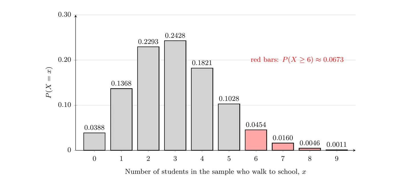
P(X = 0) = \binom{20}{0}(0.15)^0(0.85)^{20} = (0.85)^{20} \approx 0.0388

Answer: (a) about 0.2293, (b) about 0.0673, (c) about 0.0388. For (b): if we took many, many random samples of 20 students from this school, about 6.7% of the samples would have 6 or more students who walk to school. (The bars for 10 or more are too short to see. Together they have probability less than 0.001.)

Mean and standard deviation of a binomial distribution

X

is binomial, its mean and standard deviation have simple formulas, both on the formula sheet:

\mu_X = np \qquad \sigma_X = \sqrt{np(1-p)}

These are shortcuts. You'd get the same answers by using the formulas from Topic 2.9 on the whole table of 21 probabilities. The mean makes intuitive sense: if 15% of students walk to school and you pick 20, you'd expect 15% of 20, which is 3, on average.

Example 3: Interpreting the mean and standard deviation

For the students who walk to school (

n = 20

p = 0.15

), calculate and interpret the mean and standard deviation of

X

\mu_X = np = 20(0.15) = 3

\sigma_X = \sqrt{np(1-p)} = \sqrt{20(0.15)(0.85)} = \sqrt{2.55} \approx 1.597

Mean: if we took many, many random samples of 20 students from this school, the average number of students per sample who walk to school would be about 3.

Standard deviation: the number of students who walk to school in random samples of 20 typically varies by about 1.60 students from the mean of 3 students.

Notice what the mean does not say. It doesn't say every sample of 20 students has exactly 3 walkers. Some have 0 or 1, and a few have 6 or more. It describes the average over all possible samples.

The shape of a binomial distribution

The shape depends on

p

(and on

n

If $p < 0.5$ , the distribution is skewed right: most of the probability is on small counts, with a tail to the right. The distribution of walkers above is skewed right.

If $p = 0.5$ , the distribution is symmetric.

If $p > 0.5$ , the distribution is skewed left.

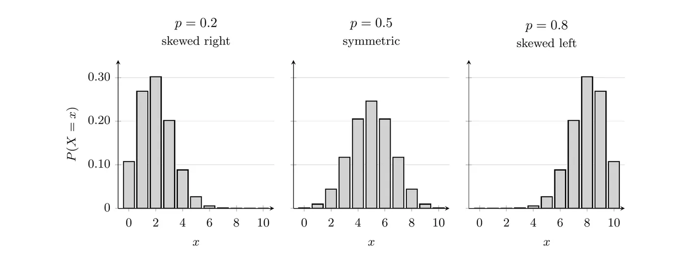
For a fixed

p

, a larger

n

makes the distribution more symmetric and bell-shaped. That idea comes back in Unit 3, where a normal model is used for proportions when the sample is large enough.

Estimating binomial probabilities with a simulation

A probability distribution can be built using the rules of probability (like the binomial formula) or estimated with a simulation (Topic 2.3). A simulation is a good way to check a formula answer. Here's a simulation for the students who walk to school:

Model one trial. Use random two-digit numbers from 00 to 99. Let 01 to 15 represent a student who walks (15 of the 100 numbers), and let 16 to 99 and 00 represent a student who doesn't, so the probability of a walker is $\frac{15}{100} = 0.15$ .

Model one sample. Generate 20 two-digit numbers and count how many are from 01 to 15. That count is one simulated value of $X$ .

Repeat. Do this many times. Here, 100 times.

Estimate. The proportion of simulated samples with $X \ge 6$ estimates $P(X \ge 6)$ .

On a TI-84, randBin(20, 0.15, 100) generates all 100 simulated counts at once. Here are the results of one simulation: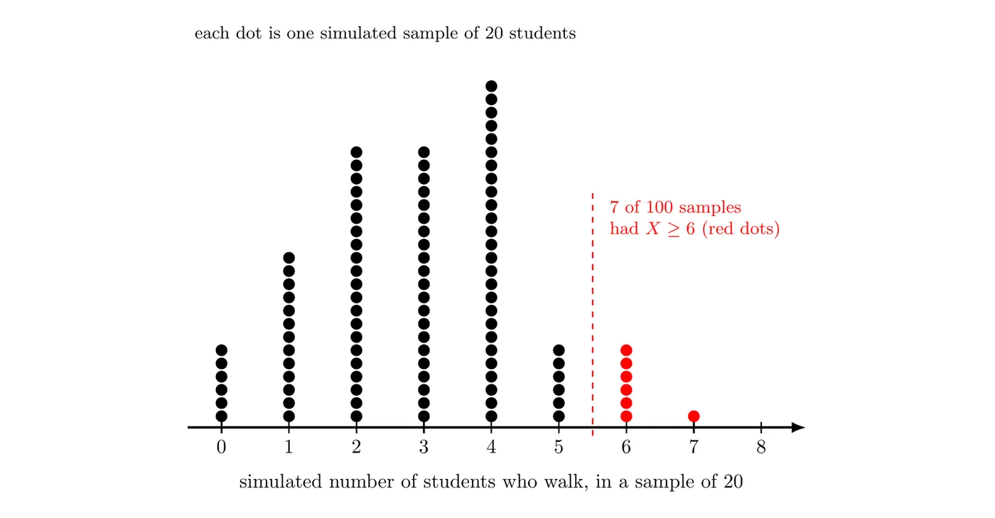

In this simulation, 7 of the 100 samples had at least 6 students who walk, so the estimate is

P(X \ge 6) \approx \frac{7}{100} = 0.07

. That's close to the exact answer of 0.0673. The average of the 100 simulated counts was 2.95, close to

\mu_X = 3

. A different simulation would give slightly different numbers, and more repetitions usually give estimates closer to the exact values.

Example 4: A taste test claim (AP-style)

Jada claims she can tell bottled water from tap water by taste. To test her, a friend fills 12 cups. For each cup, a coin flip decides whether it gets bottled or tap water, and Jada tastes it and says which one she thinks it is. She gets 10 of the 12 right.

(a) Suppose Jada is only guessing. Let

X

= the number she gets right. Explain why

X

is binomial and give

n

and

p

. (b) If she's only guessing, find the probability that she gets 10 or more right. (c) Does her result give convincing evidence that she can taste the difference? Explain.

(a) Each guess is right or wrong (binary). The water in each cup is set by a separate coin flip, so one guess doesn't change the chance of being right on another (independent). There are

n = 12

cups (number). A pure guess is right with probability

p = 0.5

on every cup (same probability). So

X

is binomial with

n = 12

and

p = 0.5

(b) "10 or more" means 10, 11, or 12:

P(X \ge 10) = \binom{12}{10}(0.5)^{12} + \binom{12}{11}(0.5)^{12} + \binom{12}{12}(0.5)^{12} = \frac{66 + 12 + 1}{4096} = \frac{79}{4096} \approx 0.0193

With a calculator:

P(X \ge 10) = 1 - P(X \le 9)

= 1

-

binomcdf(12, 0.5, 9)

\approx 0.0193

(c) Yes. If Jada were only guessing, she would get 10 or more right only about 1.9% of the time. That's unlikely to happen by chance alone, so her result gives convincing evidence that she can tell the difference. It doesn't prove it, though. A lucky guesser could still do this about 2 times in 100. Asking "how likely is a result this extreme if only chance is at work?" is the idea behind significance tests in Unit 3.

Common mistakes

Calling something binomial without checking. Go through BINS in context every time. No fixed $n$ , or trials that affect each other, means it's not binomial.

Mixing up pdf and cdf. binompdf gives exactly $x$ . binomcdf gives $x$ or fewer.

Off-by-one errors. $P(X \ge 6) = 1 - P(X \le 5)$ , not $1 - P(X \le 6)$ . Write the event out before you calculate.

Writing only calculator syntax. Name the distribution, $n$ , $p$ , and the event, then give the answer.

Forgetting the square root in $\sigma_X = \sqrt{np(1-p)}$ .

Reading the mean as a guarantee. $\mu_X = 3$ doesn't mean every sample of 20 students has exactly 3 students who walk to school.

Back Next