3.15 - Carrying Out a Chi-Square Test for Homogeneity or Independence

Overview

This topic carries out the chi-square tests set up in Topic 3.14. You compute the expected counts, the

\chi^2

statistic, the degrees of freedom, and the

p

-value, then interpret the

p

-value, make a decision, and write a conclusion in context. The four steps (State, Plan, Do, Conclude) are the same as for every test in this unit.

Expected counts

The expected count in a cell is the count you'd expect if

H_0

were true:

\text{expected count} = \frac{(\text{row total})(\text{column total})}{\text{table total}}

Why the formula works:

Homogeneity: if $H_0$ is true, every group has the same distribution, and the best estimate of it is the table's overall column proportions. In the commuting data below, 291 of all 450 adults drive, so you'd expect $\frac{291}{450}$ of City A's 120 adults to drive: $120 \cdot \frac{291}{450} = 77.6$ . That's (row total)(column total) / (table total).

Independence: if the two variables are independent, $P(\text{row and column}) = P(\text{row}) \cdot P(\text{column})$ . Multiply by the sample size $n$ : $n \cdot \frac{\text{row total}}{n} \cdot \frac{\text{column total}}{n} = \frac{(\text{row total})(\text{column total})}{n}$ .

Two good habits: keep expected counts as decimals (don't round them to whole numbers), and check that each row and column of expected counts adds up to the same totals as the observed table.

The test statistic and degrees of freedom

The test statistic for a chi-square test for homogeneity or independence is

\chi^2 = \sum \frac{(\text{Observed Count} - \text{Expected Count})^2}{\text{Expected Count}}

where the sum is taken over all cells of the two-way table (a table with 3 rows and 3 columns has 9 terms). Each term is called a component. When

H_0

is true and the conditions are met, the

\chi^2

statistic has (approximately) a chi-square distribution with

\text{df} = (\text{number of rows} - 1)(\text{number of columns} - 1)

Count only the rows and columns of categories, not the totals. Why this df? For a table with

r

rows and

c

columns, once the row and column totals are fixed, only

(r - 1)(c - 1)

cells can be filled in freely; the totals force the rest. In a 3 by 3 table, once the 4 cells of the top-left 2 by 2 block are filled in, the totals determine every other cell.

Finding the $p$ -value

The

p

-value is the area to the right of the observed

\chi^2

under the chi-square curve with the right df. It's always the right tail, and it's never doubled.

Table C: go to the row for your df, see where your $\chi^2$ falls among the critical values, and read the tail probabilities at the top of those columns. For df = 4 and $\chi^2 = 17.58$ : 17.58 is between 16.42 (tail probability 0.0025) and 18.47 (tail probability 0.001), so $0.001 < p\text{-value} < 0.0025$ .

TI-84, the whole test: enter the observed counts (no totals) in matrix [A] using 2nd, $x^{-1}$ (MATRIX), EDIT. Then STAT, TESTS, χ²-Test, with Observed: [A] and Expected: [B], and Calculate. It reports $\chi^2$ , the $p$ -value, and df, and it stores the expected counts in [B] so you can check the condition.

TI-84, just the area: χ²cdf(lower, 1E99, df).

On the exam, write the formula with the first few terms filled in, then report

\chi^2

, df, and the

p

-value.

Interpreting the $p$ -value

The

p

-value is the probability of getting a

\chi^2

statistic as large as or larger than the one observed, assuming

H_0

is true. The interpretation must state that assumption in context:

Assuming [ $H_0$ in context], there is a [ $p$ -value] probability of getting a $\chi^2$ statistic of [observed value] or larger by chance.

Making the decision and the conclusion

Compare the

p

-value to

\alpha

in writing. If the

p

-value

\leq \alpha

, reject

H_0

. If the

p

-value

> \alpha

, fail to reject

H_0

The test's result is the statistical reasoning that answers the investigative question about the population (independence) or the populations (homogeneity). State the conclusion in context, in terms of

H_a

, with non-definitive language, and name the population or populations:

Homogeneity, reject $H_0$ : there is convincing evidence that the distributions of [variable] differ across [the populations].

Independence, reject $H_0$ : there is convincing evidence of an association between [variable 1] and [variable 2] in [the population].

Fail to reject $H_0$ : there is not convincing evidence of a difference in the distributions (or of an association). Don't write "the distributions are the same" or "the variables are independent." That's accepting $H_0$ .

Following up: which cells matter most

A significant chi-square test says the distributions differ (or the variables are associated), but not how. To describe the difference, look at the components. The cells with the largest components are where observed and expected counts differ the most. Then say whether each of those observed counts was above or below its expected count. AP questions often ask for exactly this.

Example 1: Commuting in three cities (AP-style)

Independent random samples of adults from three large cities (each with more than 200,000 adults) gave these counts for main way of commuting. Do the data give convincing evidence, at

\alpha = 0.05

, that the distribution of commuting method differs among the three cities?

City	Car	Public transit	Bike or walk	Total
City A	78	30	12	120
City B	84	48	18	150
City C	129	24	27	180
Total	291	102	57	450

State:

$H_0$ : There is no difference in the distributions of main commuting method for adults in City A, City B, and City C.

$H_a$ : There is a difference in the distributions of main commuting method for adults in City A, City B, and City C.

Use

\alpha = 0.05

Plan: Chi-square test for homogeneity. Check the conditions:

Randomization: independent random samples of adults from the three cities.

10%: each sample (120, 150, and 180 adults) is less than 10% of its city's more than 200,000 adults.

Expected counts: all are greater than 5 (the smallest is $\frac{(120)(57)}{450} = 15.2$ ).

Do: Expected counts, each equal to (row total)(column total) / 450:

City	Car	Public transit	Bike or walk
City A	77.6	27.2	15.2
City B	97.0	34.0	19.0
City C	116.4	40.8	22.8

\chi^2 = \frac{(78 - 77.6)^2}{77.6} + \frac{(30 - 27.2)^2}{27.2} + \frac{(12 - 15.2)^2}{15.2} + \cdots + \frac{(27 - 22.8)^2}{22.8}

The nine components are:

City	Car	Public transit	Bike or walk
City A	0.002	0.288	0.674
City B	1.742	5.765	0.053
City C	1.364	6.918	0.774

\chi^2 \approx 17.58 \qquad \text{df} = (3 - 1)(3 - 1) = 4 \qquad p\text{-value} = P(\chi^2 \geq 17.58) \approx 0.0015

Table C agrees: in the df = 4 row, 17.58 falls between 16.42 and 18.47, so the

p

-value is between 0.001 and 0.0025.

Interpret the

p

-value: Assuming the distributions of main commuting method are the same for adults in all three cities, there is about a 0.0015 probability of getting a

\chi^2

statistic of 17.58 or larger by chance in the random sampling.

Conclude: Because the

p

-value of 0.0015 is less than

\alpha = 0.05

, we reject

H_0

. There is convincing evidence that the distributions of main commuting method differ among adults in City A, City B, and City C.

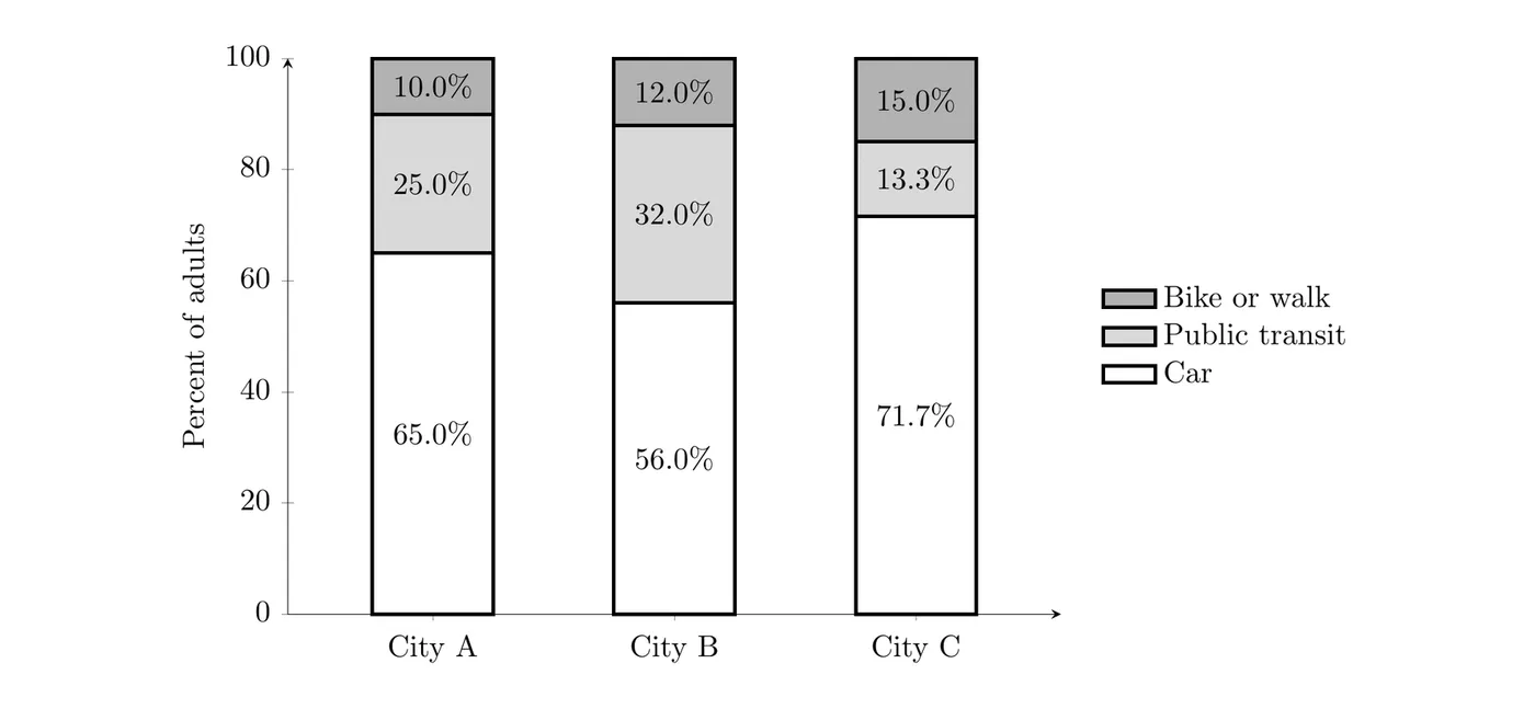
Follow-up: The two largest components are both for public transit: City C (6.918, with 24 observed versus 40.8 expected) and City B (5.765, with 48 observed versus 34.0 expected). The biggest difference is that adults in City B use public transit more than expected and adults in City C use it less. The segmented bar chart of each city's distribution shows the same pattern.

3.15 - Carrying Out a Chi-Square Test for Homogeneity or Independence

Example 2: Grade level and clubs

A random sample of 200 of the 2,400 students at a high school gave these counts. Is there convincing evidence, at

\alpha = 0.05

, of an association between grade level and number of clubs for students at this school?

Grade	None	One	Two or more	Total
9	24	19	9	52
10	20	20	10	50
11	16	20	12	48
12	13	21	16	50
Total	73	80	47	200

State:

$H_0$ : There is no association between grade level and number of clubs for students at this high school.

$H_a$ : There is an association between grade level and number of clubs for students at this high school.

Use

\alpha = 0.05

Plan: Chi-square test for independence. Check the conditions:

Randomization: a random sample of 200 students from the school.

10%: $200 \leq 10\%(2{,}400) = 240$ .

Expected counts: all are greater than 5 (the smallest is $\frac{(48)(47)}{200} = 11.28$ ).

Do: Expected counts, each equal to (row total)(column total) / 200:

Grade	None	One	Two or more
9	18.98	20.80	12.22
10	18.25	20.00	11.75
11	17.52	19.20	11.28
12	18.25	20.00	11.75

\chi^2 = \frac{(24 - 18.98)^2}{18.98} + \frac{(19 - 20.80)^2}{20.80} + \cdots + \frac{(16 - 11.75)^2}{11.75} \approx 6.07

\text{df} = (4 - 1)(3 - 1) = 6 \qquad p\text{-value} = P(\chi^2 \geq 6.07) \approx 0.415

Table C agrees: in the df = 6 row, 6.07 is less than 7.84 (tail probability 0.25), so the

p

-value is greater than 0.25.

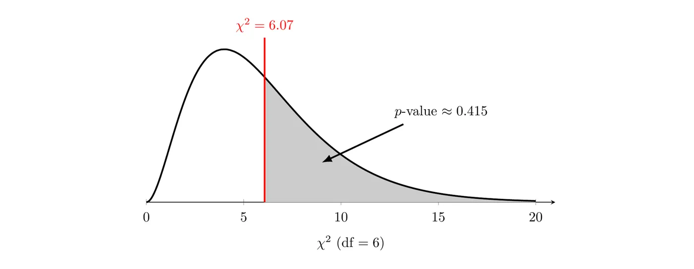
Interpret the

p

-value: Assuming there is no association between grade level and number of clubs for students at this school, there is about a 0.415 probability of getting a

\chi^2

statistic of 6.07 or larger by chance in the random sampling.

Conclude: Because the

p

-value of 0.415 is greater than

\alpha = 0.05

, we fail to reject

H_0

. There is not convincing evidence of an association between grade level and number of clubs for students at this high school.

The sample does show a small pattern (32% of the seniors were in two or more clubs, compared with 17% of the ninth graders), but a pattern that size could easily come from random sampling alone. That's why the conclusion says "not convincing evidence" instead of "no association."

Common mistakes

Rounding expected counts to whole numbers. Keep the decimals.

Wrong df: using $n - 1$ , or counting the total row and column. Use $(r - 1)(c - 1)$ with the category rows and columns only.

Doubling the $p$ -value. A chi-square $p$ -value is always one right tail.

Using proportions or percentages in the formula instead of counts.

Accepting $H_0$ : writing "the variables are independent" or "the distributions are the same" after failing to reject.

Saying the test shows which group differs. The test only says a difference exists. Use the components and the observed counts to describe it.

Leaving "assuming $H_0$ is true" out of the $p$ -value interpretation.

Back Next