5.3 - Concentration Changes Over Time

Overview

Topic 5.2 found rate laws by comparing initial rates from separate trials. This topic finds the order from a single trial: you follow one reactant's concentration as it falls over time and see which graph of the data is a straight line. The slope of that line gives the rate constant. It also covers half-life and radioactive decay.

Integrated rate laws

A rate law tells you the rate at given concentrations. An integrated rate law tells you the concentration at a given time. For a reaction where reactant A is used up, the AP reference sheet gives one for each order:

	Zero order	First order	Second order
Rate law	rate $= k$	rate $= k[\mathrm{A}]$	rate $= k[\mathrm{A}]^2$
Integrated rate law	$[\mathrm{A}]_t - [\mathrm{A}]_0 = -kt$	$\ln[\mathrm{A}]_t - \ln[\mathrm{A}]_0 = -kt$	$\dfrac{1}{[\mathrm{A}]_t} - \dfrac{1}{[\mathrm{A}]_0} = kt$
Straight-line graph	$[\mathrm{A}]$ vs. $t$	$\ln[\mathrm{A}]$ vs. $t$	$1/[\mathrm{A}]$ vs. $t$
Slope of that line	$-k$	$-k$	$+k$
Units of $k$	M/s	$\mathrm{s^{-1}}$	$\mathrm{M^{-1}\,s^{-1}}$
Half-life	Gets shorter as the reaction goes	Constant: $t_{1/2} = 0.693/k$	Gets longer as the reaction goes

Here

[\mathrm{A}]_0

is the starting concentration and

[\mathrm{A}]_t

is the concentration at time

t

. Rate here means how fast A itself is used up,

-\Delta[\mathrm{A}]/\Delta t

, even if A's coefficient isn't 1. That's how the AP exam uses these equations. Each integrated rate law is the equation of a line in disguise. Rearrange the first-order one:

\ln[\mathrm{A}]_t = -kt + \ln[\mathrm{A}]_0 \qquad \text{compare with} \qquad y = mx + b

So a graph of

\ln[\mathrm{A}]

(the

y

) against

t

(the

x

) is a line with slope

-k

and

y

-intercept

\ln[\mathrm{A}]_0

. The zero- and second-order equations work the same way (see the table).

Reading the order from a graph of [A] vs. time

A graph of reactant concentration against time already tells you a lot. In the graph below, three reactions start at the same concentration and with the same initial rate, but they quickly spread apart.

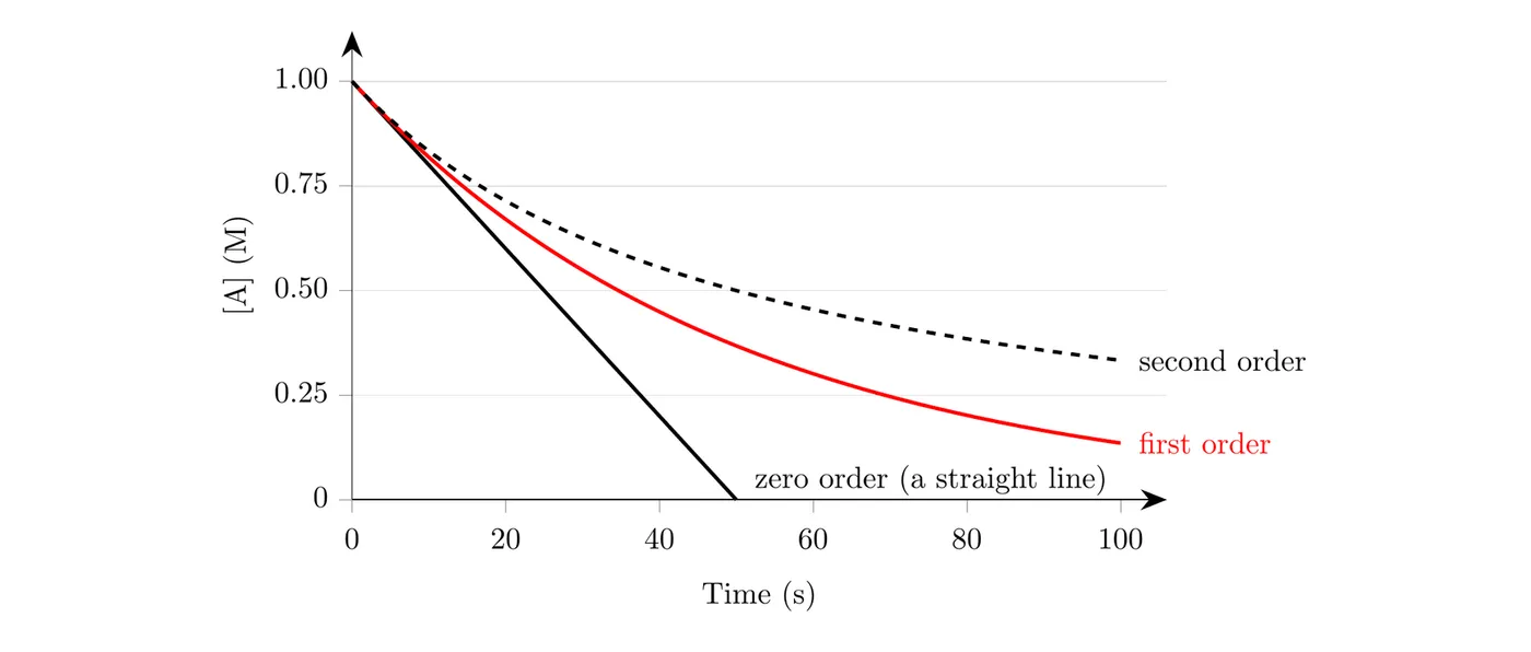
Zero order: a straight line. The rate doesn't depend on $[\mathrm{A}]$ , so the concentration drops by the same amount every second until A runs out.

First order: a curve that gets less steep over time, with the same half-life wherever you start.

Second order: a curve that starts the same way but levels off more, because the rate depends on $[\mathrm{A}]^2$ and drops fast as A is used up. Each half-life is longer than the one before.

A straight line means zero order. A curve means first or second order. To decide which, graph

\ln[\mathrm{A}]

and

1/[\mathrm{A}]

against time and see which one is straight.

First-order reactions: ln[A] vs. time is linear

If a reaction is first order with respect to the reactant you're monitoring, a graph of the natural log of its concentration against time is a straight line with slope

-k

. (In the examples on this page, the reactions and their orders are real, but the concentrations and rate constants are made up.)

Example 1: Fading of crystal violet

In the crystal violet lab from Topic 5.2,

\mathrm{CV^+}

reacts with a large excess of hydroxide ion:

\mathrm{CV^+(aq) + OH^-(aq) \rightarrow CVOH(aq)}

A spectrophotometer gives the concentrations below, and the last two columns are calculated from them. Find the order with respect to

\mathrm{CV^+}

, the rate constant, and the half-life.

Time (s)	$[\mathrm{CV^+}]$ (M)	$\ln[\mathrm{CV^+}]$	$1/[\mathrm{CV^+}]$ ( $\mathrm{M^{-1}}$ )
0	$2.50 \times 10^{-5}$	$-10.597$	$4.00 \times 10^{4}$
100	$1.98 \times 10^{-5}$	$-10.830$	$5.05 \times 10^{4}$
200	$1.57 \times 10^{-5}$	$-11.062$	$6.37 \times 10^{4}$
300	$1.25 \times 10^{-5}$	$-11.290$	$8.00 \times 10^{4}$
400	$9.92 \times 10^{-6}$	$-11.521$	$1.01 \times 10^{5}$
500	$7.87 \times 10^{-6}$	$-11.752$	$1.27 \times 10^{5}$
600	$6.25 \times 10^{-6}$	$-11.983$	$1.60 \times 10^{5}$

Graph each column against time:

Only

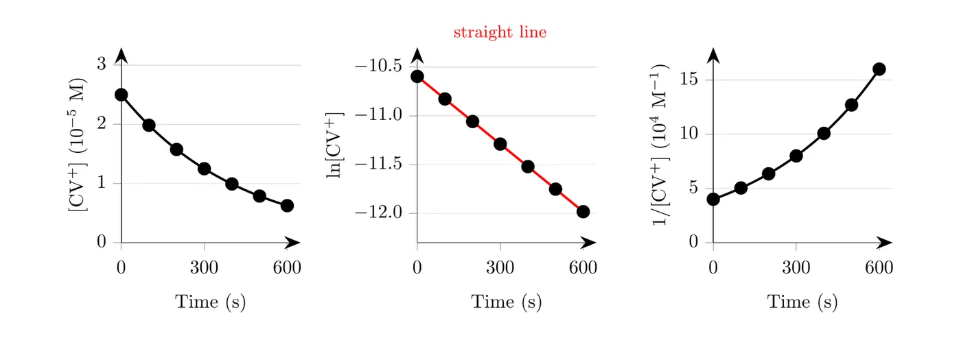
\ln[\mathrm{CV^+}]

vs. time is a straight line, so the reaction is first order with respect to

\mathrm{CV^+}

. Find the slope from the first and last points:

\text{slope} = \frac{-11.983 - (-10.597)}{600\ \mathrm{s} - 0\ \mathrm{s}} = -2.31 \times 10^{-3}\ \mathrm{s^{-1}}

Since the slope is

-k

k = 2.31 \times 10^{-3}\ \mathrm{s^{-1}}

. Then the half-life is:

t_{1/2} = \frac{0.693}{k} = \frac{0.693}{2.31 \times 10^{-3}\ \mathrm{s^{-1}}} = 3.00 \times 10^{2}\ \mathrm{s}

The table agrees:

[\mathrm{CV^+}]

falls from

2.50 \times 10^{-5}

M to

1.25 \times 10^{-5}

M in the first 300 s, then to

6.25 \times 10^{-6}

M in the next 300 s.

Lab note:

\mathrm{OH^-}

is in large excess, so its concentration barely changes, and the

k

you get includes the effect of that fixed

[\mathrm{OH^-}]

. A second run with a different

[\mathrm{OH^-}]

would show its order. Since absorbance is proportional to concentration, you can also find

k

straight from a graph of

\ln A

vs. time.

Second-order reactions: 1/[A] vs. time is linear

If a reaction is second order with respect to the reactant you're monitoring, a graph of

1/[\mathrm{A}]

against time is a straight line with slope

+k

. The slope is positive because

1/[\mathrm{A}]

gets bigger as

[\mathrm{A}]

gets smaller.

Example 2: Decomposition of nitrogen dioxide

At a certain temperature, nitrogen dioxide decomposes:

\mathrm{2NO_2(g) \rightarrow 2NO(g) + O_2(g)}

Time (s)	$[\mathrm{NO_2}]$ (M)	$\ln[\mathrm{NO_2}]$	$1/[\mathrm{NO_2}]$ ( $\mathrm{M^{-1}}$ )
0	0.0100	$-4.605$	$1.00 \times 10^{2}$
100	0.00667	$-5.010$	$1.50 \times 10^{2}$
200	0.00500	$-5.298$	$2.00 \times 10^{2}$
300	0.00400	$-5.521$	$2.50 \times 10^{2}$
400	0.00333	$-5.705$	$3.00 \times 10^{2}$
500	0.00286	$-5.857$	$3.50 \times 10^{2}$
600	0.00250	$-5.991$	$4.00 \times 10^{2}$

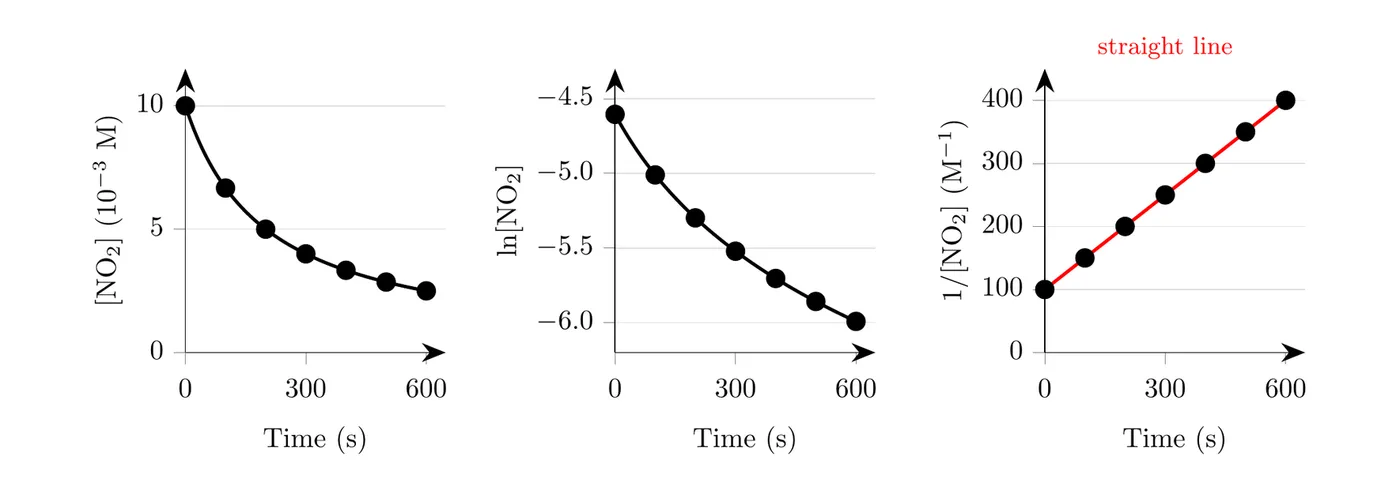
This time only

1/[\mathrm{NO_2}]

vs. time is straight, so the reaction is second order in

\mathrm{NO_2}

, with rate

= k[\mathrm{NO_2}]^2

. The slope is

k

k = \text{slope} = \frac{(4.00 \times 10^{2} - 1.00 \times 10^{2})\ \mathrm{M^{-1}}}{600\ \mathrm{s} - 0\ \mathrm{s}} = 0.500\ \mathrm{M^{-1}\,s^{-1}}

The half-life isn't constant here.

[\mathrm{NO_2}]

takes 200 s to fall from 0.0100 M to 0.00500 M, then 400 s more to fall to 0.00250 M. A half-life that keeps growing is another sign of second order.

Zero-order reactions: [A] vs. time is linear

A zero-order reaction runs at a constant rate (rate

= k

), so

[\mathrm{A}]

drops along a straight line with slope

-k

. This happens when something other than the reactant's concentration limits the rate. A classic case is a gas reacting on a hot metal surface: once the surface is completely covered, adding more gas can't speed things up.

Example 3: Ammonia on hot tungsten

Ammonia decomposes on a hot tungsten wire:

\mathrm{2NH_3(g) \rightarrow N_2(g) + 3H_2(g)}

Time (s)	$[\mathrm{NH_3}]$ (M)
0	0.00800
500	0.00675
1000	0.00550
1500	0.00425
2000	0.00300

Find the order and the rate constant.

Every 500 s,

[\mathrm{NH_3}]

drops by the same 0.00125 M. A constant drop means a straight line on a graph of

[\mathrm{NH_3}]

vs. time, so the reaction is zero order. The slope is

-k

\text{slope} = \frac{0.00300\ \mathrm{M} - 0.00800\ \mathrm{M}}{2000\ \mathrm{s} - 0\ \mathrm{s}} = -2.50 \times 10^{-6}\ \mathrm{M/s} \quad\Rightarrow\quad k = 2.50 \times 10^{-6}\ \mathrm{M/s}

The rate law is rate

= k

, and the units of

k

(M/s) fit a zero-order reaction. The half-lives shrink: going from 0.00800 M to 0.00400 M takes 1600 s, but from 0.00400 M to 0.00200 M takes only 800 s.

Half-life

The half-life,

t_{1/2}

, is the time it takes for a reactant's concentration to fall to half of its value. For a first-order reaction, set

[\mathrm{A}]_t = \tfrac{1}{2}[\mathrm{A}]_0

in the integrated rate law:

\ln\left(\tfrac{1}{2}[\mathrm{A}]_0\right) - \ln[\mathrm{A}]_0 = -kt_{1/2} \quad\Rightarrow\quad \ln\tfrac{1}{2} = -kt_{1/2} \quad\Rightarrow\quad t_{1/2} = \frac{\ln 2}{k} = \frac{0.693}{k}

The starting concentration cancels out. That's why the half-life of a first-order reaction is constant: it takes as long to go from 1.00 M to 0.500 M as from 0.0100 M to 0.00500 M. After

n

half-lives, the fraction left is

(\tfrac{1}{2})^n

Radioactive decay

Radioactive decay is the classic first-order process. Every unstable nucleus has the same chance of decaying in any second, no matter how many others are around, so the decay rate is proportional to the number of nuclei present. The half-life of an isotope doesn't depend on how much of it you have, and unlike a chemical reaction, it isn't changed by temperature.

Since

\ln[\mathrm{A}]_t - \ln[\mathrm{A}]_0 = \ln([\mathrm{A}]_t/[\mathrm{A}]_0)

depends only on a ratio, you can use mass, moles, or number of atoms in place of concentration.

Example 4: Iodine-131

Iodine-131, used to treat thyroid disease, has a half-life of 8.02 days. A hospital receives a 20.0 mg sample. (a) How much is left after 24.06 days? (b) Find

k

. (c) How much is left after 30.0 days?

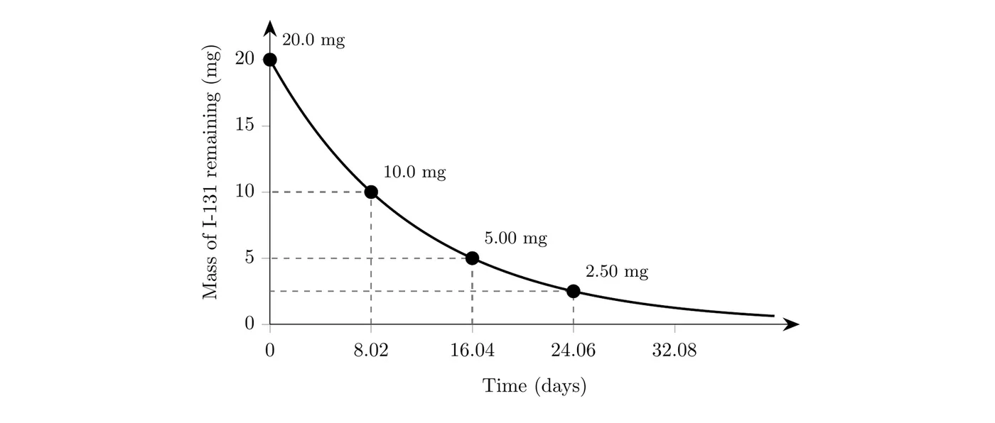
(a) 24.06 days is

24.06/8.02 = 3

half-lives: 20.0 mg to 10.0 mg to 5.00 mg to 2.50 mg. So 2.50 mg is left.

(b)

k = \frac{0.693}{t_{1/2}} = \frac{0.693}{8.02\ \mathrm{days}} = 0.0864\ \mathrm{day^{-1}}

(c) 30.0 days isn't a whole number of half-lives, so use the integrated rate law with masses (

m

in mg):

\ln m_t = \ln(20.0) - (0.0864\ \mathrm{day^{-1}})(30.0\ \mathrm{days}) = 2.996 - 2.592 = 0.404

m_t = e^{0.404} = 1.50\ \mathrm{mg}

Check: 30.0 days is just under 4 half-lives, so the answer should be just over

20.0/16 = 1.25

mg. It is.

Example 5: Reading a first-order graph (AP-style)

Hydrogen peroxide decomposes in the presence of a catalyst:

\mathrm{2H_2O_2(aq) \rightarrow 2H_2O(l) + O_2(g)}

The graph shows

\ln[\mathrm{H_2O_2}]

vs. time for one trial.

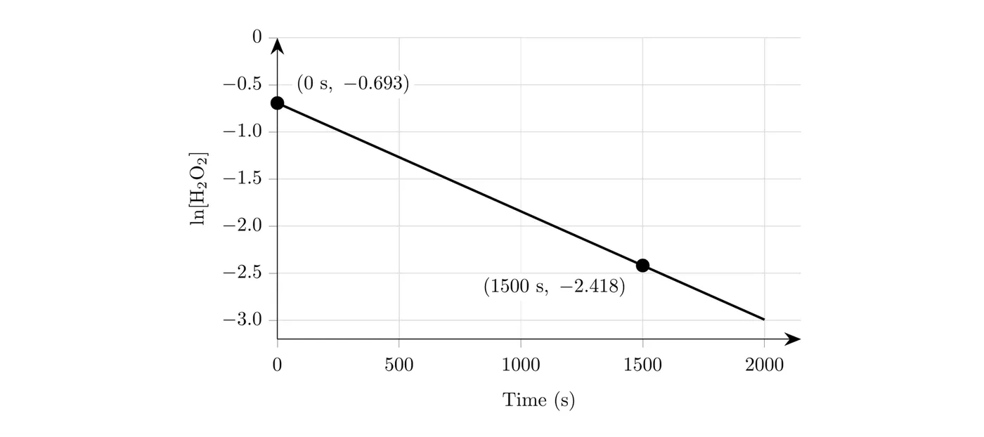
(a) What is the order of the reaction with respect to

\mathrm{H_2O_2}

? Justify your answer. (b) Determine

k

, with units. (c) Calculate the half-life. (d) What is

[\mathrm{H_2O_2}]

at 1500 s? (e) Calculate the initial rate of disappearance of

\mathrm{H_2O_2}

(a) First order. The graph of

\ln[\mathrm{H_2O_2}]

vs. time is a straight line, which happens only when the reaction is first order in the reactant being monitored.

(b) Use the two labeled points:

\text{slope} = \frac{-2.418 - (-0.693)}{1500\ \mathrm{s} - 0\ \mathrm{s}} = -1.15 \times 10^{-3}\ \mathrm{s^{-1}}

The slope is

-k

, so

k = 1.15 \times 10^{-3}\ \mathrm{s^{-1}}

. The units

\mathrm{s^{-1}}

fit a first-order reaction.

(c)

t_{1/2} = \frac{0.693}{1.15 \times 10^{-3}\ \mathrm{s^{-1}}} = 603\ \mathrm{s}

(d) At 1500 s,

\ln[\mathrm{H_2O_2}] = -2.418

, so:

[\mathrm{H_2O_2}] = e^{-2.418} = 0.0891\ \mathrm{M}

(e) First find the starting concentration from the

y

-intercept:

[\mathrm{H_2O_2}]_0 = e^{-0.693} = 0.500

M. Then use the rate law:

\text{rate} = k[\mathrm{H_2O_2}]_0 = (1.15 \times 10^{-3}\ \mathrm{s^{-1}})(0.500\ \mathrm{M}) = 5.75 \times 10^{-4}\ \mathrm{M/s}

Common mistakes

Mixing up the slopes. The slope is $-k$ for the zero- and first-order graphs and $+k$ for the second-order graph. $k$ itself is always positive.

Using log instead of ln. The integrated rate law uses the natural log (the LN key on a calculator).

Using $t_{1/2} = 0.693/k$ for any order. It's only for first order. For other orders the half-life changes as the reaction goes.

Confusing graph units with the balanced equation. The axes are concentration (M), $\ln$ of concentration (no units), or $1/$ concentration ( $\mathrm{M^{-1}}$ ), against time. The coefficients in the balanced equation don't appear on them.

Back Next