3.1 - Estimators

Overview

You almost never get to measure a whole population, so you use a sample to estimate the number you care about. This topic names the pieces (parameters, statistics, and estimators) and gives you the main test of a good estimator: is it unbiased? Every confidence interval and significance test in Units 3 and 4 is built on these ideas.

Point estimators and point estimates

Recall from Topic 1.2: a parameter is a number that describes a whole population (usually unknown), and a statistic is a number calculated from a sample. Inference uses statistics to estimate parameters.

A sample statistic is a point estimator of the matching population parameter, and you can think of its value as the estimate of that parameter. "Point" means a single number, as opposed to an interval (which starts in Topic 3.3). For example, the sample proportion

\hat{p}

is a point estimator for the population proportion

p

. These are the estimators Units 3 and 4 use:

Quantity	Parameter (population)	Point estimator (sample statistic)
Proportion	$p$	$\hat{p}$ ("p-hat")
Mean	$\mu$	$\bar{x}$ ("x-bar")
Standard deviation	$\sigma$	$s$
Difference in proportions	$p_1 - p_2$	$\hat{p}_1 - \hat{p}_2$
Difference in means	$\mu_1 - \mu_2$	$\bar{x}_1 - \bar{x}_2$

Strictly speaking, the estimator is the rule (for example, "divide the number of successes by

n

"), and the estimate is the number you get when you apply the rule to your sample. On the exam you'll usually calculate the estimate and say which parameter it estimates.

The sample proportion is

\hat{p} = \frac{\text{number of successes in the sample}}{n}

where

n

is the sample size. A "success" is just the outcome you're counting. It doesn't have to be something good.

Example 1: Estimating a population proportion

Suppose a city council wants to know what proportion of the city's registered voters support a new library tax. It surveys a random sample of 250 registered voters, and 145 say they support the tax. Identify the parameter, and calculate a point estimate for it.

Step 1: Identify the parameter.

p

= the proportion of all registered voters in the city who support the library tax.

Step 2: Calculate the matching statistic.

\hat{p} = \frac{145}{250} = 0.58

Answer: The point estimate is

\hat{p} = 0.58

. Our best single guess is that about 58% of all registered voters in the city support the library tax.

Example 2: Estimating a mean and a standard deviation

A random sample of 8 employees at a large company recorded their one-way commute times, in minutes: 12, 25, 18, 30, 22, 15, 27, 19. Calculate point estimates for the mean

\mu

and the standard deviation

\sigma

of commute times for all employees at the company.

Step 1: The sample mean

\bar{x}

estimates

\mu

\bar{x} = \frac{12 + 25 + 18 + 30 + 22 + 15 + 27 + 19}{8} = \frac{168}{8} = 21 \text{ minutes}

Step 2: The sample standard deviation

s

estimates

\sigma

. The deviations from 21 are

-9, 4, -3, 9, 1, -6, 6, -2

, and their squares add up to

81 + 16 + 9 + 81 + 1 + 36 + 36 + 4 = 264

s = \sqrt{\frac{\sum (x_i - \bar{x})^2}{n - 1}} = \sqrt{\frac{264}{7}} \approx 6.14 \text{ minutes}

Answer: The point estimates are

\bar{x} = 21

minutes for

\mu

and

s \approx 6.14

minutes for

\sigma

. On a TI-84, enter the data in L1 and run STAT > CALC > 1-Var Stats. It reports

\bar{x}

and Sx, which is

s

Unbiased estimators

Different samples give different values of a statistic. That's sampling variability, and it's expected. So the question isn't whether one estimate is exactly right (it almost never is). The question is whether the estimator is right on average.

When estimating a population parameter, an estimator is unbiased if, on average, its value does not underestimate or overestimate the parameter. Picture taking every possible sample of the same size and calculating the statistic each time: for an unbiased estimator, the mean of all those values (the center of its sampling distribution) equals the parameter. An estimator is biased if its sampling distribution is centered somewhere else, so it tends to land too high or too low.

Think of a dart player. Unbiased means the darts are centered on the bullseye, even if they're spread out. Biased means they're centered somewhere off the bullseye, no matter how tightly they're grouped.

Bias and variability are different things

Bias is about the center of the sampling distribution: is it at the parameter?

Variability is about the spread of the sampling distribution: how much do the estimates change from sample to sample?

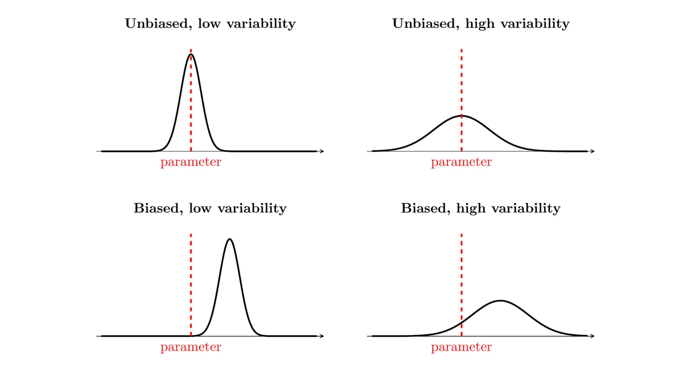
The best estimator is unbiased with low variability (top left). Larger random samples reduce variability, but they don't fix bias. A biased method gives a biased answer at any sample size.

Common unbiased (and biased) estimators

$\hat{p}$ is an unbiased estimator of $p$ . Topic 3.2 shows why: the mean of the sampling distribution of $\hat{p}$ is exactly $p$ .

$\bar{x}$ is an unbiased estimator of $\mu$ .

The sample variance $s^2$ is an unbiased estimator of $\sigma^2$ . That's why its formula divides by $n - 1$ instead of $n$ : dividing by $n$ would underestimate $\sigma^2$ on average.

The sample maximum is a biased estimator of the population maximum. A sample can't contain a value larger than the population's largest value, so it can only miss on the low side. The sample range is biased low for the same reason.

How to justify bias on the AP exam

You'll usually see a simulated sampling distribution (a dotplot or histogram of many values of the estimator) along with the true value of the parameter. Then:

Find the center of the simulated values (their mean, or by eye).

Compare that center to the parameter.

If the center is about equal to the parameter, the estimator appears unbiased. If it's clearly above or below, the estimator is biased, and you say in which direction.

Always talk about the center of the distribution of the estimator, not about one single estimate.

Example 3: Choosing between two estimators (AP-style)

A box holds tickets numbered 1, 2, 3, and so on up to

N

, and you want to estimate

N

, the largest number. You draw a random sample of 5 tickets without replacement. Two estimators are proposed:

Estimator A: the sample maximum (the largest number you drew).

Estimator B: $2\bar{x} - 1$ , where $\bar{x}$ is the mean of your 5 numbers. The mean of the numbers 1 to $N$ is $\frac{N + 1}{2}$ , so this estimator is built to hit $N$ on average.

To compare them, a student sets

N = 60

and simulates 1,000 random samples of 5 tickets, calculating both estimators for each sample. The results are below.

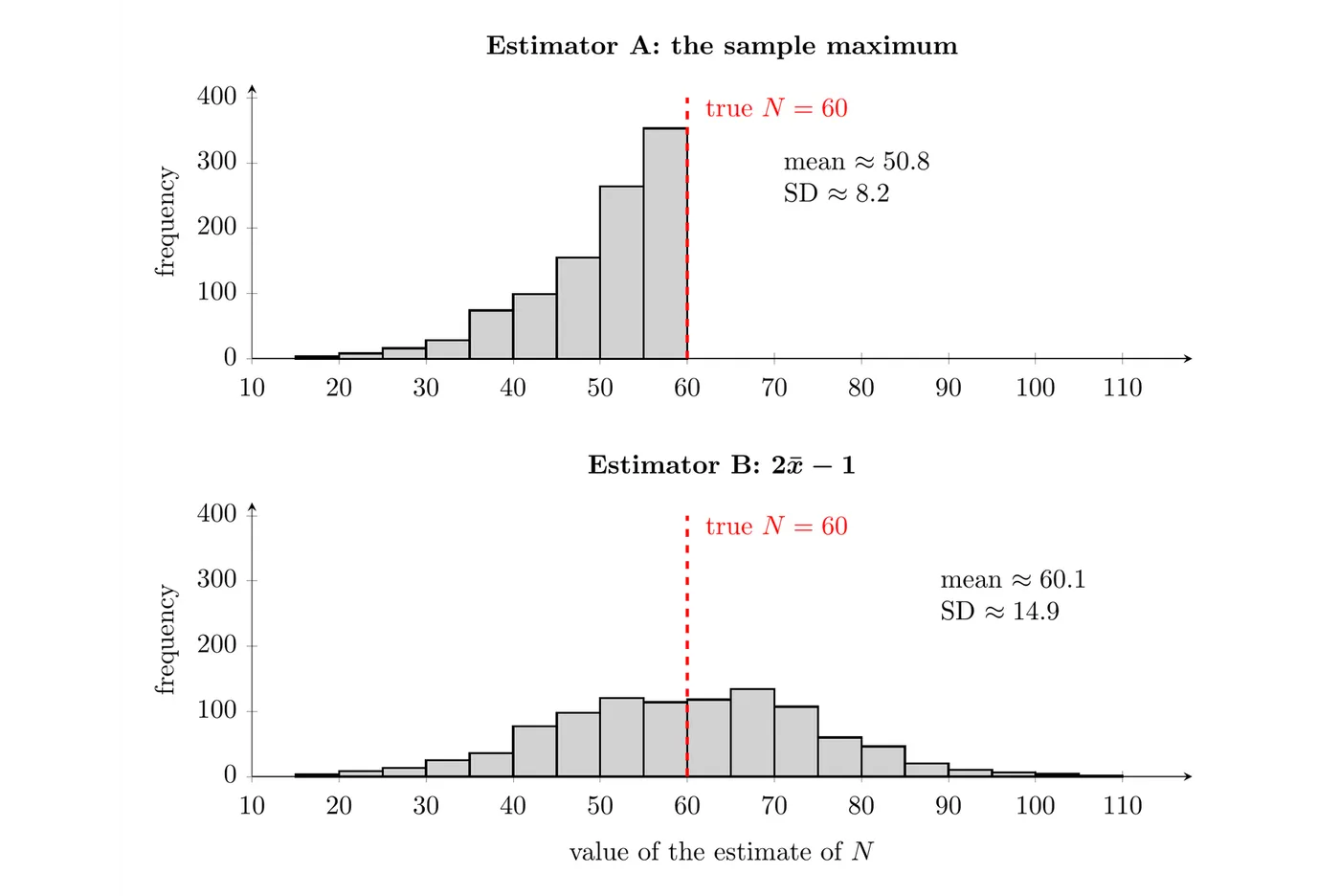
(a) Does each estimator appear to be unbiased? Justify your answer.

(b) Which estimator would you prefer? Explain.

Part (a): The 1,000 values of Estimator A have a mean of about 50.8, well below the true value

N = 60

. In fact, 915 of the 1,000 values were below 60 and none were above it, since the sample maximum can never exceed the largest ticket. Estimator A is biased: it tends to underestimate

N

The values of Estimator B have a mean of about 60.1, very close to

N = 60

, and they land above and below 60 about equally. Estimator B appears unbiased.

Part (b): Estimator A has less variability (a standard deviation of about 8.2, compared to about 14.9 for B), but it misses low by about 9 on average, and that systematic miss never goes away. Estimator B is right on average, so it's the better choice here, even though its individual estimates are more spread out. In general, you want an estimator that is unbiased and has as little variability as possible.

Common mistakes

Mixing up parameters and statistics. If the number comes from the sample you have, it's a statistic. If it describes the whole population, it's a parameter.

Thinking unbiased means accurate every time. An unbiased estimator still misses on almost every sample. It just doesn't miss in one direction on average.

Calling a single estimate biased. Bias describes the estimator (the method), based on its whole sampling distribution.

Thinking a larger sample removes bias. It only reduces variability. A biased method, like a voluntary response survey (Topic 1.12), stays biased at any size.

Comparing to the wrong value. Judge bias by comparing the center of the sampling distribution to the parameter, not to one sample's statistic.

Back Next