1.3 - Rates of Change in Linear and Quadratic Functions

Overview

Average rates of change can tell function types apart. For a linear function, the average rate of change never changes. For a quadratic function, it does change, but at a steady rate. In this topic you'll see why, connect the average rate of change to the slope of a secant line, and use changing rates to decide whether a graph is concave up or concave down.

Average rate of change is the slope of a secant line

A secant line is a line through two points on a graph. The average rate of change of

f

over

[a, b]

is the slope of the secant line from

(a, f(a))

(b, f(b))

\text{slope of secant line} = \frac{f(b) - f(a)}{b - a}

So every time you compute an average rate of change, you're finding a slope. For example, here is the secant line for

f(x) = x^2 - 4x + 5

over

[1, 4]

. Since

f(1) = 2

and

f(4) = 5

\frac{f(4) - f(1)}{4 - 1} = \frac{5 - 2}{3} = 1

1.3 - Rates of Change in Linear and Quadratic Functions

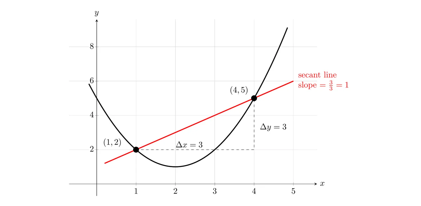
The secant line rises

3

units over a run of

3

units, so its slope, which is the average rate of change of

f

over

[1, 4]

, is

1

Linear functions: A constant rate of change

For a linear function

f(x) = mx + b

, the average rate of change over any interval, of any length, is the same number

m

\frac{f(x_2) - f(x_1)}{x_2 - x_1} = \frac{(mx_2 + b) - (mx_1 + b)}{x_2 - x_1} = \frac{m(x_2 - x_1)}{x_2 - x_1} = m

For example, look at

g(x) = -2x + 7

at equally spaced inputs:

$x$	$0$	$1$	$2$	$3$	$4$
$g(x)$	$7$	$5$	$3$	$1$	$-1$

Every output drops by

2

, so every average rate of change over these intervals is

-2

. Since the average rates of change over consecutive equal-length intervals are constant, they are changing at a rate of zero. That's the signature of a linear function.

Quadratic functions: Rates that change at a constant rate

For a quadratic function, the average rate of change is not constant. But over consecutive equal-length intervals, the average rates of change follow a linear pattern, so they change by the same amount each step.

Example 1: Average rates of change of a quadratic

Let

f(x) = x^2 - 4x + 5

. Find the average rates of change over

[0, 1]

[1, 2]

[2, 3]

[3, 4]

, and

[4, 5]

The outputs are

f(0) = 5

f(1) = 2

f(2) = 1

f(3) = 2

f(4) = 5

, and

f(5) = 10

. Each interval has length

1

Interval	Average rate of change	Change from the previous rate
$[0, 1]$	$\frac{2 - 5}{1} = -3$
$[1, 2]$	$\frac{1 - 2}{1} = -1$	$+2$
$[2, 3]$	$\frac{2 - 1}{1} = 1$	$+2$
$[3, 4]$	$\frac{5 - 2}{1} = 3$	$+2$
$[4, 5]$	$\frac{10 - 5}{1} = 5$	$+2$

Each red segment below is a secant line, labeled with its slope:

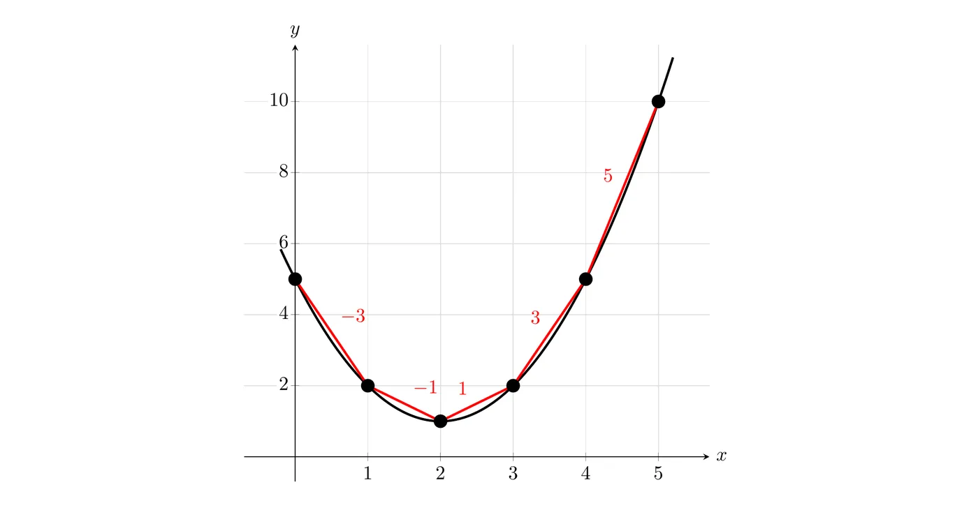
Answer: the average rates of change are

-3, -1, 1, 3, 5

. Each is

2

more than the one before, so the average rates of change are changing at a constant rate of

2

per interval. In fact, the average rate of change over

[k, k + 1]

is given by the linear function

r(k) = 2k - 3

Why this works for every quadratic

Take any quadratic

f(x) = ax^2 + bx + c

and any interval length

h

. The average rate of change from

x

x + h

is:

\frac{f(x + h) - f(x)}{h} = \frac{a(x + h)^2 + b(x + h) + c - (ax^2 + bx + c)}{h}

= \frac{2axh + ah^2 + bh}{h} = 2ax + ah + b

With

h

fixed, this is a linear function of

x

with slope

2a

. Moving to the next interval adds

h

x

, so each new average rate of change is

2ah

more than the last. For

f(x) = x^2 - 4x + 5

with

h = 1

, that's

2(1)(1) = 2

, which matches the table.

Other functions and sequences

For other function types, neither pattern holds. For

f(x) = x^3

x = 0, 1, 2, 3, 4

, the average rates of change over the unit intervals are

1, 7, 19, 37

. They aren't constant, and they don't change by a constant amount either: the changes are

6, 12, 18

. In Topic 1.5 you'll see that a cubic needs one more round of differences before the pattern turns constant.

A sequence is also a function: its inputs are the term numbers

n = 1, 2, 3, \ldots

, so the same ideas apply. The average rate of change from term

n_1

to term

n_2

\frac{a_{n_2} - a_{n_1}}{n_2 - n_1}

$4, 7, 10, 13, \ldots$ : each term is $3$ more than the last, so the average rate of change is a constant $3$ per term. That's a linear pattern (you'll call it an arithmetic sequence in Unit 2).

$2, 5, 10, 17, 26, \ldots$ : the changes are $3, 5, 7, 9$ , which go up by $2$ each step. That's a quadratic pattern. (These terms are $a_n = n^2 + 1$ .)

Concavity from average rates of change

Average rates of change over equal-length intervals also reveal concavity:

If the average rates of change over equal-length intervals are increasing (for all small intervals), the graph is concave up.

If they are decreasing, the graph is concave down.

This matches Topic 1.1: concave up means the rate of change is increasing. In Example 1, the rates

-3, -1, 1, 3, 5

increase, and the parabola opens up. For any quadratic, the rates change by

2ah

each step, so the graph is concave up everywhere when

a > 0

and concave down everywhere when

a < 0

Example 2: A growing plant (AP-style)

The height of a plant,

h(t)

, in centimeters, is measured every

2

weeks. The results are in the table.

$t$ (weeks)	$0$	$2$	$4$	$6$	$8$
$h(t)$ (centimeters)	$10$	$18$	$24$	$28$	$30$

(a) Find the average rate of change of

h

over each consecutive interval in the table. (b) Is the graph of

h

concave up or concave down on

0 \le t \le 8

? Give a reason. (c) Is a linear model or a quadratic model more appropriate for these data? Give a reason.

(a) Each interval has length

2

, so divide each change in height by

2

Interval	Average rate of change (cm per week)
$[0, 2]$	$\frac{18 - 10}{2} = 4$
$[2, 4]$	$\frac{24 - 18}{2} = 3$
$[4, 6]$	$\frac{28 - 24}{2} = 2$
$[6, 8]$	$\frac{30 - 28}{2} = 1$

(b) The average rates of change over consecutive equal-length intervals,

4, 3, 2, 1

centimeters per week, are decreasing. So the graph of

h

is concave down. In context, the plant keeps growing, but more slowly as time goes on.

(c) The average rates of change are not constant, so a linear model doesn't fit. They decrease by exactly

1

from each interval to the next, so they change at a constant rate, which is the pattern of a quadratic function. A quadratic model is more appropriate. (In fact,

h(t) = -\frac{1}{4}t^2 + \frac{9}{2}t + 10

matches every value in the table.)

Common mistakes

Using unequal intervals. The linear and quadratic patterns only show up over equal-length intervals. Check the spacing of the inputs before you compare rates.

Confusing the rates with the change in the rates. For a quadratic, the average rates of change are not constant. The change from one rate to the next is.

Getting concavity backward with negative rates. Rates of $-5, -3, -1$ are increasing, so the graph is concave up, even though every rate is negative.

Forgetting to divide by the interval length. If the inputs go up by $2$ , divide each change in output by $2$ .

Back Next