1.6 - Polynomial Functions and End Behavior

Overview

End behavior describes what a function's outputs do as the inputs head off to the far right (

x \to \infty

) or the far left (

x \to -\infty

). For a polynomial, one term decides it: the leading term. In this topic you'll describe end behavior with limit notation, see why the leading term wins, and read degree and sign clues off a graph. AP questions use this all the time, from matching a graph to its equation to writing limits on a free response question.

What end behavior means

As the inputs of a nonconstant polynomial increase without bound (get bigger and bigger with no ceiling), the outputs do one of two things: they increase without bound or they decrease without bound. They never settle down at a number. The same is true as the inputs decrease without bound (head toward the far left).

We write this with limit notation:

\lim_{x \to \infty} p(x) = \infty \quad \text{or} \quad \lim_{x \to \infty} p(x) = -\infty

\lim_{x \to -\infty} p(x) = \infty \quad \text{or} \quad \lim_{x \to -\infty} p(x) = -\infty

Notation	What it means	Graph
$\lim_{x \to \infty} p(x) = \infty$	As $x$ increases without bound, $p(x)$ increases without bound	right end rises
$\lim_{x \to \infty} p(x) = -\infty$	As $x$ increases without bound, $p(x)$ decreases without bound	right end falls
$\lim_{x \to -\infty} p(x) = \infty$	As $x$ decreases without bound, $p(x)$ increases without bound	left end rises
$\lim_{x \to -\infty} p(x) = -\infty$	As $x$ decreases without bound, $p(x)$ decreases without bound	left end falls

Here

\infty

isn't a number the outputs reach. Writing

= \infty

is shorthand for “grows without bound.”

Why nonconstant? A constant polynomial like

p(x) = 7

just stays at 7 forever. Every polynomial of degree 1 or higher heads to

\infty

-\infty

on each end, which also means a nonconstant polynomial never has a horizontal asymptote.

Why the leading term decides

Recall from Topic 1.4 that the leading term of a polynomial is the term with the highest power of

x

, written

a_n x^n

. Its coefficient

a_n

is the leading coefficient, and

n

is the degree.

|x|

gets large, higher powers grow much faster than lower powers. So for inputs of large magnitude, the leading term's values dominate (are far bigger in size than) all the lower-degree terms put together, and the polynomial acts like its leading term.

A numerical look

Take

h(x) = x^4 - 50x^3

and compare the two terms:

$x$	$x^4$	$-50x^3$	$h(x)$
$10$	$10{,}000$	$-50{,}000$	$-40{,}000$
$50$	$6{,}250{,}000$	$-6{,}250{,}000$	$0$
$100$	$100{,}000{,}000$	$-50{,}000{,}000$	$50{,}000{,}000$
$1{,}000$	$1 \times 10^{12}$	$-5 \times 10^{10}$	$9.5 \times 10^{11}$

x = 10

, the

-50x^3

term is bigger in size, so

h(10)

is negative. By

x = 100

the leading term has taken over, and by

x = 1{,}000

the

-50x^3

term barely matters. Factoring out the leading term shows why:

h(x) = x^4\left(1 - \frac{50}{x}\right)

x \to \infty

\frac{50}{x} \to 0

, so the part in parentheses approaches 1 and

h(x)

behaves like

x^4

. The same factoring works for any polynomial:

p(x) = a_n x^n\left(1 + \frac{a_{n-1}}{a_n x} + \frac{a_{n-2}}{a_n x^2} + \cdots + \frac{a_0}{a_n x^n}\right)

Every fraction inside the parentheses goes to 0 as

|x|

grows, so

p(x)

behaves like

a_n x^n

for inputs of large magnitude.

Zoom out and a polynomial looks like its leading term

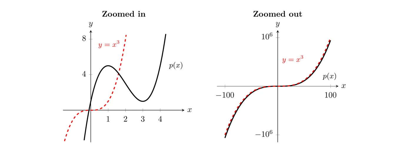
1.6 - Polynomial Functions and End Behavior

Both panels show

p(x) = x^3 - 6x^2 + 9x + 1

(black) and its leading term

y = x^3

(red, dashed). Up close they look nothing alike:

p

has a local maximum at

(1, 5)

and a local minimum at

(3, 1)

. Zoomed out to

-100 \le x \le 100

, the two graphs almost sit on top of each other. That's the leading term dominating.

The four cases

Only two facts about the leading term matter for end behavior: whether the degree is even or odd, and whether the leading coefficient is positive or negative.

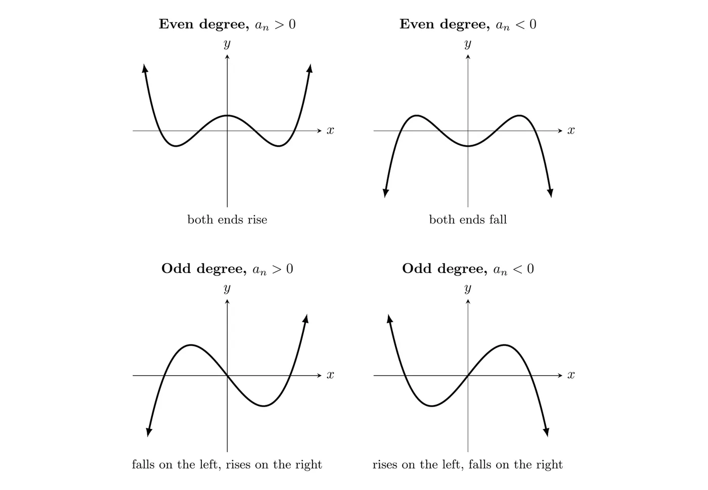
Degree	Leading coefficient	As $x \to -\infty$	As $x \to \infty$	Ends like
Even	Positive	$p(x) \to \infty$	$p(x) \to \infty$	$y = x^2$
Even	Negative	$p(x) \to -\infty$	$p(x) \to -\infty$	$y = -x^2$
Odd	Positive	$p(x) \to -\infty$	$p(x) \to \infty$	$y = x^3$
Odd	Negative	$p(x) \to \infty$	$p(x) \to -\infty$	$y = -x^3$

Why the pattern works: for large positive

x

x^n

is positive for every

n

. For large negative

x

x^n

is positive when

n

is even and negative when

n

is odd. Then multiply by the sign of

a_n

. A negative leading coefficient flips the graph over the

x

-axis, so both ends flip.

An easy way to remember: picture

y = x^2

(both ends up) and

y = x^3

(down on the left, up on the right). Every polynomial's ends look like one of those, or one of those flipped.

Leading terms in factored form

AP questions often give a polynomial in factored form. You don't need to multiply it all out. Take the highest-power term of each factor (raised to that factor's power) and multiply those together. The result is the leading term of the whole polynomial.

Watch for factors written “backward,” like

(3 - x)

. Its highest-power term is

-x

, not

x

, and that negative sign flips the end behavior.

Reading end behavior from a graph or table

You can also work backward from a graph:

Both ends go the same direction: the degree is even.

The ends go opposite directions: the degree is odd.

The right end rises: the leading coefficient is positive. The right end falls: the leading coefficient is negative.

The right end alone tells you the sign of

a_n

, because

x^n > 0

for large positive

x

no matter what

n

is.

A table can suggest end behavior too, but be careful. A table only shows a few inputs, and lower-degree terms can win for moderate inputs (see Example 3).

A useful consequence

Every odd-degree polynomial has at least one real zero. Topic 1.5 showed this with conjugate pairs, and end behavior shows it too: one end is below the

x

-axis and the other is above it, and a polynomial's graph has no breaks, so it has to cross the

x

-axis somewhere in between.

Examples

Example 1: Finding the leading term

Describe the end behavior of

q(x) = 6x^2 + 4 - 3x^7

using limit notation.

Step 1: Find the leading term, the term with the highest power of

x

. It's

-3x^7

, even though it's written last: degree 7 (odd), leading coefficient

-3

(negative).

Step 2: Odd degree with a negative leading coefficient means the graph rises on the left and falls on the right, like

y = -x^3

\lim_{x \to -\infty} q(x) = \infty, \qquad \lim_{x \to \infty} q(x) = -\infty

Answer: As

x

decreases without bound,

q(x)

increases without bound, and as

x

increases without bound,

q(x)

decreases without bound.

Example 2: Factored form

Describe the end behavior of

f(x) = (3 - x)(x + 2)^2(2x - 1)

Step 1: Take the highest-power term of each factor.

$(3 - x)$ gives $-x$

$(x + 2)^2$ gives $x^2$

$(2x - 1)$ gives $2x$

Step 2: Multiply them to get the leading term.

(-x)(x^2)(2x) = -2x^4

Step 3: Degree 4 is even, and

-2

is negative, so both ends fall.

\lim_{x \to -\infty} f(x) = -\infty, \qquad \lim_{x \to \infty} f(x) = -\infty

Answer: Both ends of the graph of

f

decrease without bound. If you'd missed the negative in

(3 - x)

, you'd have gotten both ends rising, which is exactly backward.

Example 3: When the leading term hasn't taken over yet

Let

h(x) = x^4 - 50x^3

. A student finds

h(10) = -40{,}000

and

h(20) = -240{,}000

and concludes that

\lim_{x \to \infty} h(x) = -\infty

. Is the student right?

Step 1: Check the leading term. It's

x^4

: even degree, positive leading coefficient. So the right end has to rise.

Step 2: Find where the leading term takes over. Factor:

h(x) = x^3(x - 50)

For every

x > 50

, both

x^3

and

x - 50

are positive, so

h(x) > 0

. For example,

h(100) = 50{,}000{,}000

\lim_{x \to \infty} h(x) = \infty

Answer: The student is wrong. End behavior is about inputs of large magnitude, and a couple of moderate inputs can't show it. The

-50x^3

term wins for

0 < x < 50

, but for

x > 50

the leading term wins and

h(x)

increases without bound.

Example 4: Reading a graph (AP-style)

The graph of a polynomial function

p

is shown. All real zeros of

p

are shown, at

x = -2

x = 1

, and

x = 3

, and the graph touches the

x

-axis at

x = 1

without crossing it.

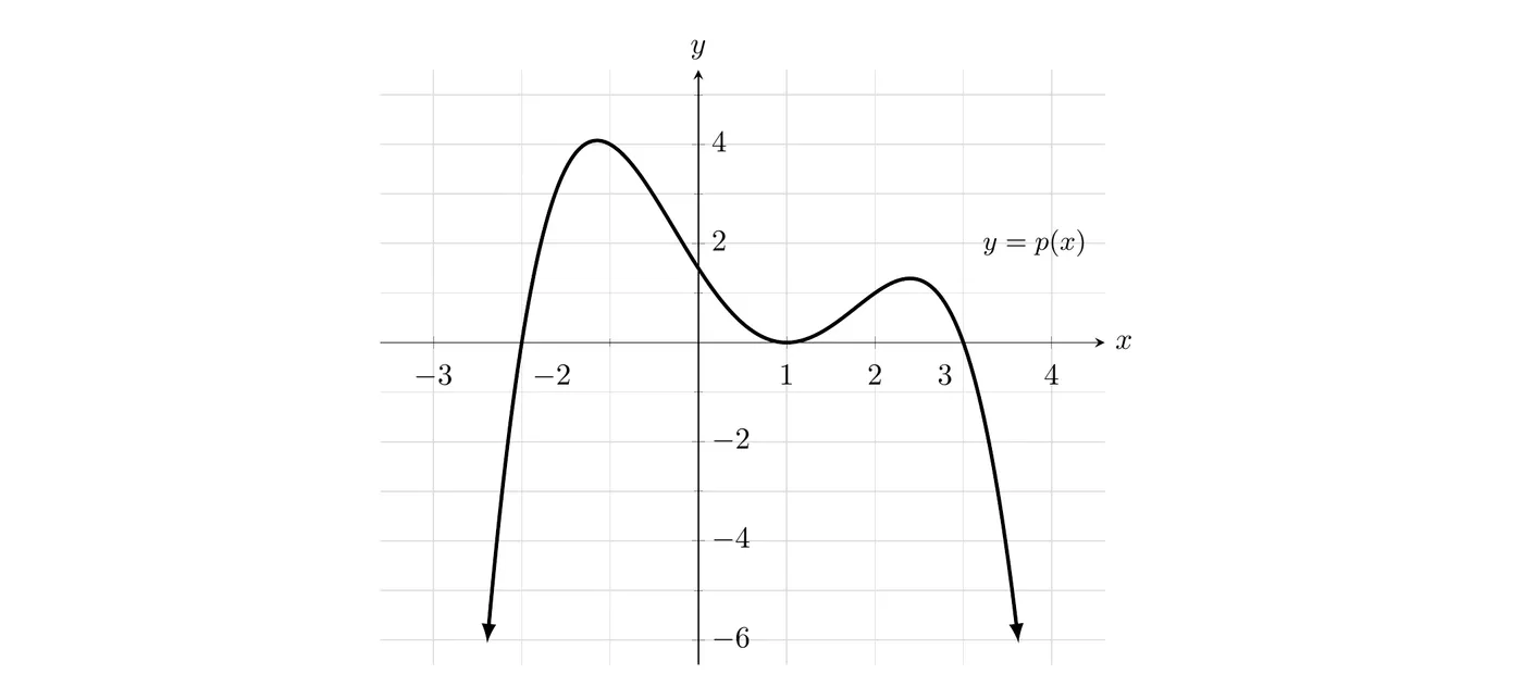
(a) Describe the end behavior of

p

using limit notation.

(b) What is the least possible degree of

p

? Is its leading coefficient positive or negative? Justify your answers.

Part (a): Both ends of the graph fall.

\lim_{x \to -\infty} p(x) = -\infty, \qquad \lim_{x \to \infty} p(x) = -\infty

Part (b): Both ends go the same way, so the degree is even. The right end falls, so the leading coefficient is negative.

For the degree, count the zeros with multiplicity (Topic 1.5). The graph crosses at

x = -2

and

x = 3

, so each has odd multiplicity, at least 1. It bounces at

x = 1

, so that zero has even multiplicity, at least 2. That's at least

1 + 2 + 1 = 4

, and 4 is even, which agrees with the end behavior.

Answer: The least possible degree is 4, and the leading coefficient is negative. One polynomial that fits is

p(x) = -\frac{1}{4}(x + 2)(x - 1)^2(x - 3)

, which is the function graphed.

Common mistakes

Using the first term written instead of the highest power. In $p(x) = 5 + 3x - x^4$ , the leading term is $-x^4$ , even though it's written last.

Losing a negative sign inside a factor like $(3 - x)$ or $(1 - 2x)$ .

Mixing up even degree with even function. $x^2 + x$ has even degree, but it isn't an even function (it's not symmetric over the $y$ -axis).

Trusting a few table values. Lower-degree terms can win for moderate inputs, as in Example 3.

Giving a polynomial a horizontal asymptote. A nonconstant polynomial never levels off.

Back Next