1.7 - Rational Functions and End Behavior

Overview

A rational function is one polynomial divided by another. Its end behavior comes down to a contest between the numerator and the denominator: for inputs of large magnitude, the one with the greater degree wins. In this topic you'll compare leading terms to find horizontal asymptotes, slant asymptotes, and polynomial-like end behavior, and describe all of it with limits.

What a rational function is

A rational function is a function that can be written as a quotient of two polynomial functions:

r(x) = \frac{p(x)}{q(x)}

where

q

is not the zero polynomial. The domain is every real number except the zeros of

q

, since you can't divide by zero. For example,

r(x) = \frac{x + 1}{x^2 - x - 6} = \frac{x + 1}{(x - 3)(x + 2)}

has domain all real numbers except

x = 3

and

x = -2

For each input in the domain,

r(x)

measures how big the numerator is compared to the denominator. If

r(5) = 3

, the numerator is three times the denominator at

x = 5

. If

r(5) = 0.01

, the numerator is tiny compared to the denominator. This relative-size idea is the key to end behavior.

Compare the leading terms

From Topic 1.6, a polynomial is dominated by its leading term for inputs of large magnitude. So for large

|x|

, a rational function behaves like the quotient of the two leading terms:

r(x) = \frac{a_n x^n + \cdots}{b_m x^m + \cdots} \quad \text{behaves like} \quad \frac{a_n x^n}{b_m x^m}

Simplify that quotient, and it tells you the end behavior. There are three cases, depending on which polynomial has the greater degree.

Case 1: The denominator dominates

If the denominator has the greater degree (

n < m

), the quotient of leading terms simplifies to a constant over a nonconstant polynomial, like

\frac{5}{x^2}

. As

|x|

grows, that shrinks toward 0. The graph has a horizontal asymptote at

y = 0

Example 1: Limits at both ends

Find

\lim_{x \to \infty} \frac{5x}{x^3 - 1}

and

\lim_{x \to -\infty} \frac{5x}{x^3 - 1}

Step 1: The degrees are 1 and 3, so the denominator dominates.

Step 2: The quotient of leading terms is

\frac{5x}{x^3} = \frac{5}{x^2}

, which goes to 0 as

|x|

grows.

\lim_{x \to \infty} \frac{5x}{x^3 - 1} = 0, \qquad \lim_{x \to -\infty} \frac{5x}{x^3 - 1} = 0

Answer: Both limits are 0, so

y = 0

is a horizontal asymptote on both ends. The denominator grows so much faster than the numerator that the fraction shrinks toward 0.

Case 2: Neither dominates

If the degrees are equal (

n = m

), the powers of

x

cancel and the quotient of leading terms is a constant: the ratio of the leading coefficients,

\frac{a_n}{b_m}

. The graph has a horizontal asymptote at

y = \frac{a_n}{b_m}

Example 2: Equal degrees

Find

\lim_{x \to \infty} \frac{3x^2 + 1}{6x^2 - 5x}

Step 1: Both degrees are 2, so neither dominates.

Step 2: The quotient of leading terms is

\frac{3x^2}{6x^2} = \frac{1}{2}

\lim_{x \to \infty} \frac{3x^2 + 1}{6x^2 - 5x} = \frac{3}{6} = \frac{1}{2}

Check with a table: the outputs creep toward 0.5.

$x$	$10$	$100$	$1{,}000$
$\frac{3x^2 + 1}{6x^2 - 5x}$	$0.5473$	$0.5042$	$0.5004$

Answer: The limit is

\frac{1}{2}

. The same is true as

x \to -\infty

, so

y = \frac{1}{2}

is a horizontal asymptote on both ends.

Case 3: The numerator dominates

If the numerator has the greater degree (

n > m

), the quotient of leading terms is a nonconstant polynomial. The rational function has the same end behavior as that polynomial, so its outputs increase or decrease without bound and there's no horizontal asymptote.

Example 3: Ends like a parabola

Describe the end behavior of

r(x) = \frac{x^4}{2x^2 + 1}

Step 1: The quotient of leading terms is

\frac{x^4}{2x^2} = \frac{1}{2}x^2

Step 2: That's an even-degree polynomial with a positive leading coefficient, so both ends rise (Topic 1.6).

\lim_{x \to -\infty} r(x) = \infty, \qquad \lim_{x \to \infty} r(x) = \infty

Answer: Both ends increase without bound, and for large

|x|

the graph looks like

y = \frac{1}{2}x^2

. For example,

r(100) \approx 4{,}999.75

, while

\frac{1}{2}(100)^2 = 5{,}000

Slant asymptotes

When the numerator's degree is exactly one more than the denominator's, the quotient of leading terms is linear, like

2x

. Then the graph has a slant asymptote (also called an oblique asymptote): a slanted line the graph gets closer and closer to as

x \to \pm\infty

. The slant asymptote is parallel to the line you get from the leading terms. To find its exact equation, divide the polynomials (polynomial long division is in Topic 1.11).

Example 4: A slant asymptote

Describe the end behavior of

r(x) = \frac{2x^2 + 3x - 1}{x - 1}

and find its slant asymptote.

Step 1: The quotient of leading terms is

\frac{2x^2}{x} = 2x

. It's linear, so there's a slant asymptote parallel to

y = 2x

, meaning it has slope 2.

Step 2: Divide to get the exact line:

\frac{2x^2 + 3x - 1}{x - 1} = 2x + 5 + \frac{4}{x - 1}

Check by multiplying back:

(x - 1)(2x + 5) + 4 = 2x^2 + 3x - 5 + 4 = 2x^2 + 3x - 1

Step 3: As

|x|

grows,

\frac{4}{x - 1} \to 0

, so the graph gets closer and closer to the line

y = 2x + 5

1.7 - Rational Functions and End Behavior

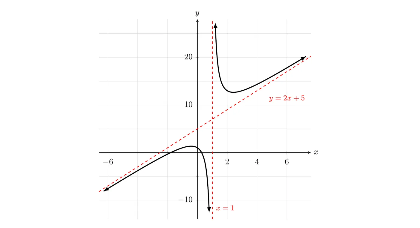
Answer: The slant asymptote is

y = 2x + 5

, and the end behavior is

\lim_{x \to -\infty} r(x) = -\infty

and

\lim_{x \to \infty} r(x) = \infty

. For large positive

x

the leftover piece

\frac{4}{x - 1}

is positive, so the graph sits just above the line; for large negative

x

it sits just below. (The dashed line

x = 1

is a vertical asymptote, which is Topic 1.9.)

Summary of the three cases

Degrees	Quotient of leading terms	End behavior
$n < m$ (denominator dominates)	A constant over a nonconstant polynomial	Horizontal asymptote $y = 0$
$n = m$ (neither dominates)	The constant $\frac{a_n}{b_m}$	Horizontal asymptote $y = \frac{a_n}{b_m}$
$n = m + 1$	Linear, $\frac{a_n}{b_m}x$	Slant asymptote parallel to $y = \frac{a_n}{b_m}x$
$n > m + 1$	A polynomial of degree 2 or more	Same end behavior as that polynomial

What a horizontal asymptote really means

If the graph of

r

has a horizontal asymptote at

y = b

, the outputs get arbitrarily close to

b

and stay arbitrarily close to

b

as the inputs increase or decrease without bound. Pick any tiny distance, like 0.001. Eventually, every output is within 0.001 of

b

. In limit notation:

\lim_{x \to \infty} r(x) = b \quad \text{or} \quad \lim_{x \to -\infty} r(x) = b

Two things that surprise students:

A graph can cross its horizontal asymptote. The asymptote only describes the ends. In the middle of the graph, anything can happen.

The graph can approach from above or below, and it can be different on the two ends.

This is

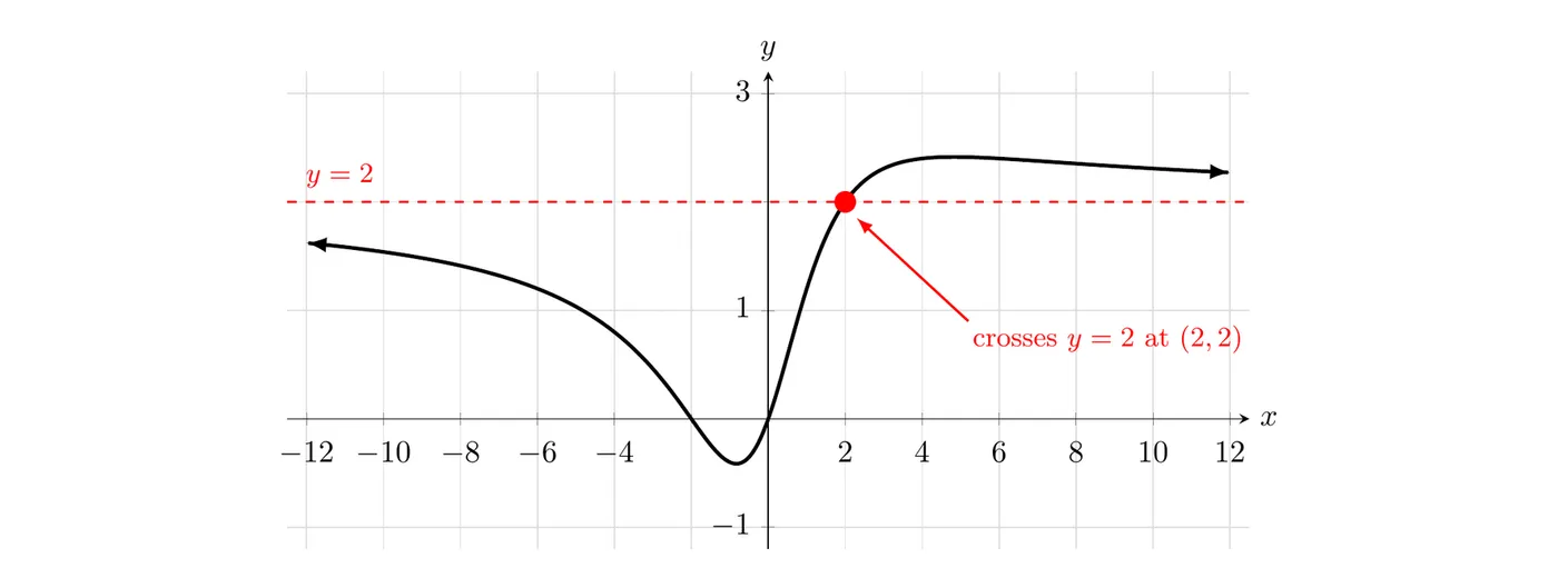
h(x) = \frac{2x^2 + 4x}{x^2 + 4}

. The degrees match, so the horizontal asymptote is

y = \frac{2}{1} = 2

. To see where the graph crosses it, solve

h(x) = 2

2x^2 + 4x = 2(x^2 + 4)

, so

4x = 8

and

x = 2

. The graph crosses its asymptote at

(2, 2)

, rises a little above it, and then settles back toward 2 from above. On the left end, it approaches 2 from below.

Example 5: Concentration in a tank (AP-style)

A large tank starts with 200 liters of pure water. Salt water with 40 grams of salt per liter flows in at 10 liters per minute, and the tank is kept well mixed (nothing flows out). After

t

minutes, the tank holds

400t

grams of salt in

200 + 10t

liters of water, so the concentration of salt is

C(t) = \frac{400t}{200 + 10t} \text{ grams per liter}

(a) Find

\lim_{t \to \infty} C(t)

and explain what it means in context.

(b) After how many minutes does the concentration stay within 1 gram per liter of that limit?

Part (a): Both the numerator and denominator have degree 1, so the limit is the ratio of the leading coefficients.

\lim_{t \to \infty} C(t) = \frac{400}{10} = 40

Over a long time, the concentration gets closer and closer to 40 grams per liter, the concentration of the incoming salt water. That makes sense: as more salt water pours in, the original 200 liters of pure water matter less and less.

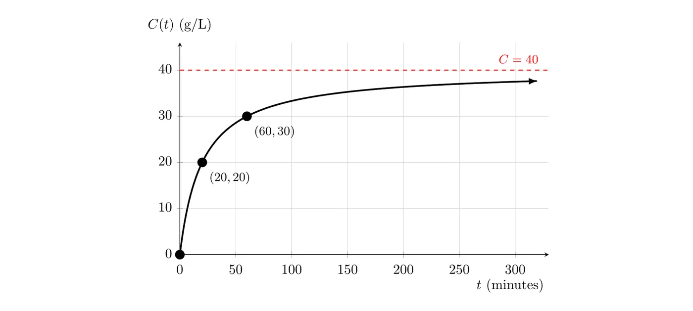
The graph shows the curve climbing toward the asymptote

C = 40

. For example,

C(20) = \frac{8{,}000}{400} = 20

and

C(60) = \frac{24{,}000}{800} = 30

Part (b): Since

C(t) < 40

for all

t \ge 0

, we need

40 - C(t) < 1

. Combine into one fraction:

40 - \frac{400t}{200 + 10t} = \frac{40(200 + 10t) - 400t}{200 + 10t} = \frac{8{,}000}{200 + 10t}

Because

200 + 10t

is positive, multiplying both sides by it keeps the inequality the same direction:

\frac{8{,}000}{200 + 10t} < 1 \;\Rightarrow\; 8{,}000 < 200 + 10t \;\Rightarrow\; t > 780

Check:

C(780) = \frac{400(780)}{200 + 7{,}800} = \frac{312{,}000}{8{,}000} = 39

, exactly 1 gram per liter below 40.

Answer: After 780 minutes (13 hours), the concentration stays within 1 gram per liter of 40 g/L. This is what “arbitrarily close” looks like in practice: for any closeness you choose, there's a time after which the concentration stays that close.

Common mistakes

Using the ratio of leading coefficients when the degrees differ. $\frac{5x}{x^3 - 1}$ has horizontal asymptote $y = 0$ , not $y = 5$ .

Thinking a graph can never cross a horizontal asymptote. It can, as $h(x)$ above does at $(2, 2)$ .

Dropping a sign. $\frac{-3x^2 + 1}{x^2 + 4}$ has horizontal asymptote $y = -3$ .

Stopping at the leading terms for a slant asymptote. The leading terms give the slope ( $y = 2x$ in Example 4). Division gives the exact line ( $y = 2x + 5$ ).

Saying “no horizontal asymptote” means there's no end behavior. There's always end behavior. Describe it with limits, like in Example 3.

Back Next