2.3 - Exponential Functions

Overview

An exponential function multiplies its output by the same factor every time the input goes up by 1. That one fact controls its whole graph: it's always increasing or always decreasing, it never changes concavity, and on one side it levels off toward a horizontal asymptote. This topic covers the general form

f(x) = ab^x

and the key features the AP exam asks you to identify.

The general form

f(x) = ab^x, \quad a \neq 0, \quad b > 0, \quad b \neq 1

$a$ is the initial value: $f(0) = ab^0 = a$ . It's the $y$ -intercept.

$b$ is the base: the factor the output is multiplied by each time $x$ goes up by 1.

Each restriction has a reason:

$b > 0$ , because a negative base breaks down for many inputs. For example, $(-4)^{1/2} = \sqrt{-4}$ isn't a real number.

$b \neq 1$ , because $1^x = 1$ for every $x$ , so $f(x) = a$ would just be a constant function.

$a \neq 0$ , because otherwise $f(x) = 0$ for every $x$ .

Two special names, both with

a > 0

Exponential growth: $a > 0$ and $b > 1$ .

Exponential decay: $a > 0$ and $0 < b < 1$ .

What the input counts

When the input is a natural number, it tells you how many factors of the base get multiplied onto the initial value. For

f(x) = 5(2)^x

f(3) = 5 \cdot \underbrace{2 \cdot 2 \cdot 2}_{3 \text{ factors}} = 40

But the domain of an exponential function is all real numbers, not just whole numbers, and other inputs still have meaning:

$f(0) = 5(2)^0 = 5$ : zero factors of 2, so just the initial value.

$f(-1) = 5(2)^{-1} = 2.5$ : a negative input divides by the base instead.

$f\left(\frac{1}{2}\right) = 5(2)^{1/2} = 5\sqrt{2} \approx 7.07$ : a fractional input applies part of a factor.

That's why the graph is one smooth, unbroken curve instead of a set of dots.

Always increasing or decreasing, never changing concavity

Because the outputs are proportional over equal-length intervals,

f(x + 1) = b \cdot f(x)

for every

x

. Take growth (

a > 0

and

b > 1

). Every step multiplies by something bigger than 1, so the function always increases. The size of each step is

f(x + 1) - f(x) = f(x)(b - 1)

which gets bigger as

f(x)

gets bigger. The rate of change keeps increasing, so the graph is concave up everywhere. The same reasoning works for the other three cases:

$a$	$b$	Increasing or decreasing	Concavity	Example
$a > 0$	$b > 1$	increasing	concave up	$y = 2^x$ (growth)
$a > 0$	$0 < b < 1$	decreasing	concave up	$y = \left(\frac{1}{2}\right)^x$ (decay)
$a < 0$	$b > 1$	decreasing	concave down	$y = -2^x$
$a < 0$	$0 < b < 1$	increasing	concave down	$y = -\left(\frac{1}{2}\right)^x$

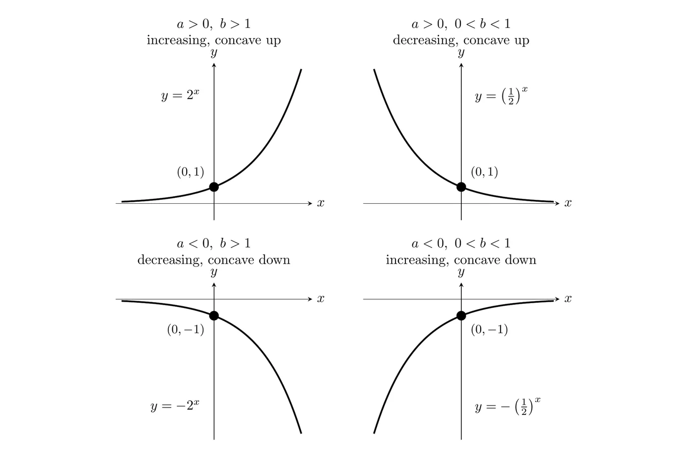
A quick way to remember it: the sign of

a

sets the concavity (positive

a

means concave up, negative

a

means concave down). When

a < 0

, the graph is a growth or decay graph flipped over the

x

-axis.

Two consequences the AP exam tests directly:

No extrema on the whole domain. An exponential function never turns around, so it has no relative or absolute maximum or minimum. On a closed interval $[p, q]$ it does have both, and they're at the endpoints.

No points of inflection. The concavity never changes, so there's no point where it switches.

Example 1: Key features from the formula

Describe the key features of

f(x) = -2(3)^x

$a = -2 < 0$ and $b = 3 > 1$ , so $f$ is decreasing and concave down.

Initial value: $f(0) = -2$ , so the $y$ -intercept is $(0, -2)$ .

Since $3^x > 0$ for every $x$ , $f(x) = -2(3)^x$ is always negative. The range is $(-\infty, 0)$ , and there are no zeros.

As $x$ increases, $3^x$ grows without bound, so $f(x)$ decreases without bound. As $x$ decreases, $3^x$ shrinks toward 0, so $f(x)$ approaches 0 from below.

Answer: decreasing, concave down,

y

-intercept

(0, -2)

, range

(-\infty, 0)

, no zeros, no extrema, and no points of inflection.

Example 2: Extrema on a closed interval

Find the maximum and minimum values of

g(x) = 8\left(\frac{1}{2}\right)^x

on the interval

[-1, 3]

Here

a = 8 > 0

and

0 < b < 1

, so

g

is always decreasing. A decreasing function is largest at the left endpoint and smallest at the right endpoint.

g(-1) = 8\left(\tfrac{1}{2}\right)^{-1} = 8(2) = 16 \qquad g(3) = 8\left(\tfrac{1}{2}\right)^{3} = \frac{8}{8} = 1

Answer: on

[-1, 3]

, the maximum value is 16 (at

x = -1

) and the minimum value is 1 (at

x = 3

). On all real numbers,

g

has no maximum or minimum.

End behavior and the horizontal asymptote

For an exponential function in general form, one end of the graph goes off to

\infty

-\infty

, and the other end gets arbitrarily close to 0. In limit notation:

Case	$\lim_{x \to \infty} ab^x$	$\lim_{x \to -\infty} ab^x$
$a > 0$ , $b > 1$	$\infty$	$0$
$a > 0$ , $0 < b < 1$	$0$	$\infty$
$a < 0$ , $b > 1$	$-\infty$	$0$
$a < 0$ , $0 < b < 1$	$0$	$-\infty$

Since one side approaches 0, the line

y = 0

(the

x

-axis) is a horizontal asymptote. The graph gets closer and closer to it but never reaches it, because

b^x

is never 0. So

f(x) = ab^x

has no zeros.

Why does

b^x

approach 0 as

x \to \infty

when

0 < b < 1

? Multiplying by a number less than 1 over and over keeps shrinking the value:

\left(\frac{1}{2}\right)^{10} \approx 0.001

and

\left(\frac{1}{2}\right)^{20} \approx 0.000001

Exponential plus a constant

Sometimes a function's outputs aren't proportional over equal-length intervals, but they become proportional after you add or subtract a constant. Then the function can be modeled by an additive transformation of an exponential function:

f(x) = ab^x + k

Adding

k

shifts the whole graph up

k

units. The horizontal asymptote moves to

y = k

, and the end behavior approaches

k

instead of 0. Whether the function increases or decreases, and its concavity, don't change.

Example 3: Finding the hidden exponential

Show that the function in the table is not of the form

ab^x

, then find a model for it.

$x$	0	1	2	3	4
$f(x)$	7	10	16	28	52

Step 1: check the ratios.

\frac{10}{7} \approx 1.43

\frac{16}{10} = 1.6

, and

\frac{28}{16} = 1.75

aren't constant, so

f

is not of the form

ab^x

Step 2: look at the differences: 3, 6, 12, 24. Each one is double the one before. For

f(x) = ab^x + k

, the constant cancels when you subtract,

f(x + 1) - f(x) = ab^{x+1} - ab^x = ab^x(b - 1)

so the differences are themselves exponential with the same base. That makes

b = 2

Step 3: find

a

and

k

. The first difference is

f(1) - f(0) = a(b - 1) = a(2 - 1) = a

, so

a = 3

. Then

f(0) = a + k

gives

7 = 3 + k

, so

k = 4

Step 4: check by subtracting 4 from every output: 3, 6, 12, 24, 48. Each value is double the one before, so

f(x) - 4 = 3(2)^x

Answer:

f(x) = 3(2)^x + 4

. Its graph is the graph of

y = 3(2)^x

shifted up 4, with horizontal asymptote

y = 4

, so

\lim_{x \to -\infty} f(x) = 4

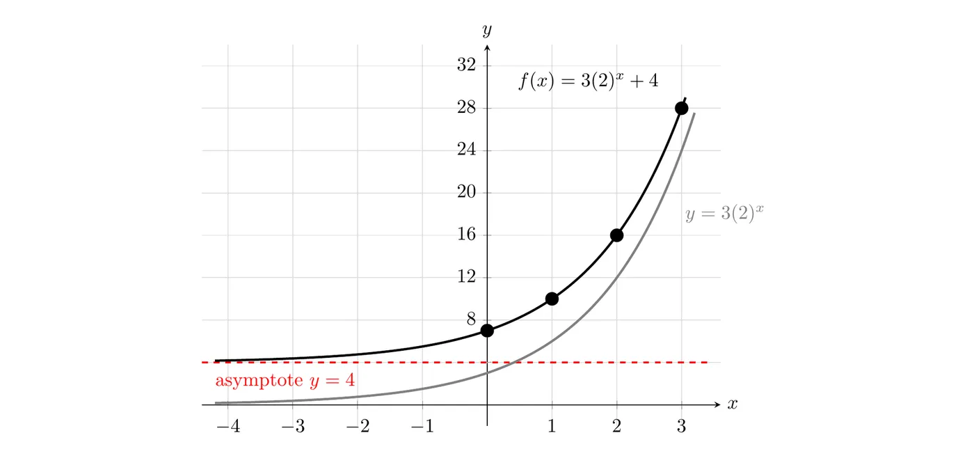
In real contexts the constant is often given to you, like room temperature for a cooling drink. You'll build models like that in Topic 2.5.

Common mistakes

Calling every decreasing exponential function decay. Decay means $a > 0$ and $0 < b < 1$ . The function $y = -3(2)^x$ decreases, but it's a growth function flipped over the $x$ -axis, not exponential decay.

Thinking the graph touches the asymptote. $ab^x$ is never 0, so the graph never crosses or touches $y = 0$ .

Claiming an extremum without a closed interval. On all real numbers, an exponential function has no maximum or minimum. The $y$ -intercept is not a minimum.

Raising the coefficient to the power. $ab^x$ is not $(ab)^x$ . In $2(3)^x$ only the 3 is raised to the power: $2(3)^2 = 18$ , but $6^2 = 36$ .

Forcing the basic form onto shifted data. If the ratios aren't constant, check whether the differences have a constant ratio, or whether subtracting a constant makes the outputs proportional, before giving up on an exponential model.

Back Next