2.6 - Competing Function Model Validation

Overview

Real data almost never follows a perfect pattern, so more than one type of function can look like a good fit. In this topic you build linear, quadratic, and exponential models for the same data set, then decide which one really fits. You use two tools to decide: the context of the data, and residuals, which measure how far off a model's predictions are.

When more than one model could work

When the rate of change in a data set changes only slightly, a linear, a quadratic, and an exponential model can all look reasonable. Over a short stretch of inputs, a gently curving exponential looks a lot like a parabola, and both look close to a line.

Each type of model leaves its own fingerprint in a table with equally spaced inputs:

Model	Form	What stays (nearly) constant	How the rate of change behaves
Linear	$f(x) = mx + b$	First differences (the change in output)	Constant
Quadratic	$f(x) = ax^2 + bx + c$	Second differences	Changes at a constant rate
Exponential	$f(x) = ab^x$	Ratios of consecutive outputs	Proportional to the output value

With real data, nothing is exactly constant. Look for the pattern that is closest to constant, then let technology build the model.

Building the models with technology

The AP exam expects you to build these models with a calculator. On a TI-84, enter the inputs in L1 and the outputs in L2 (STAT, then EDIT). Then press STAT, go to CALC, and pick the regression:

LinReg(ax+b) for a linear model

QuadReg for a quadratic model

ExpReg for an exponential model of the form $y = ab^x$

Other graphing tools, like Desmos, do the same thing with a table and a regression equation.

Example 1: Spotting the candidate models

The table shows the number of users

y

, in thousands, of a new study app

x

months after it launched. Which types of models are reasonable for this data?

$x$ (months)	0	1	2	3	4	5	6	7
$y$ (thousands)	40.3	44.6	49.7	56.4	63.3	70.2	79.1	88.2

Step 1: First differences. Subtract each output from the next one:

4.3,\ 5.1,\ 6.7,\ 6.9,\ 6.9,\ 8.9,\ 9.1

These aren't constant. They mostly grow, so the rate of change is increasing and a line will miss some of the curve.

Step 2: Second differences. Subtract consecutive first differences:

0.8,\ 1.6,\ 0.2,\ 0.0,\ 2.0,\ 0.2

These bounce around a lot, so the quadratic pattern isn't very clean.

Step 3: Ratios. Divide each output by the one before it:

\frac{44.6}{40.3} \approx 1.107,\ 1.114,\ 1.135,\ 1.122,\ 1.109,\ 1.127,\ 1.115

These all stay close to

1.12

Answer: The rate of change only changes slightly, so all three types are candidates. The ratios are the closest to constant, which points toward an exponential model. Running the regressions (rounded) gives:

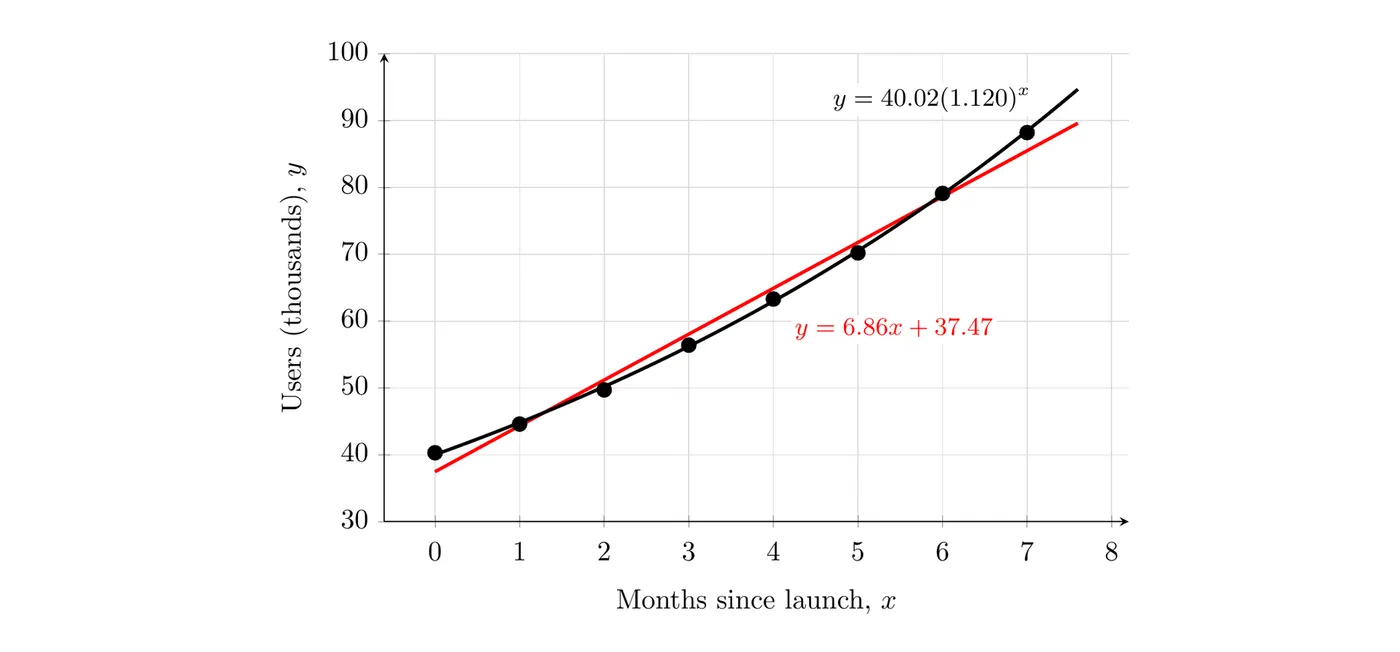
\text{Linear: } y = 6.86x + 37.47 \qquad \text{Exponential: } y = 40.02(1.120)^x

2.6 - Competing Function Model Validation

Both models hug the data, so the graph alone can't settle it. Context and residuals can.

Choosing a model using context

Models can be compared using clues from the context. Ask what the situation says about how the quantity changes.

Clue in the context	Model it suggests
The quantity changes by the same amount each period (a fixed fee per mile, water pumped at a steady rate)	Linear
The rate of change itself changes steadily, or the quantity rises then falls with one maximum or minimum (the height of a thrown ball, profit as a price goes up)	Quadratic
The quantity changes by the same percent or factor each period (interest, population growth, radioactive decay)	Exponential

Also think about what each model does outside the data:

A decreasing linear model eventually predicts negative values. That makes no sense for something like a population or a mass.

A quadratic model eventually turns around. If nothing in the context would make the quantity turn around, that's a warning sign.

An exponential model grows without bound or decays toward a horizontal asymptote. Decay toward 0 fits things like a medicine leaving the bloodstream.

For the app, users tend to invite their friends, so the number of new users each month is roughly proportional to the number of current users. That's growth by a constant percent (about

12\%

per month), which is exponential. A quadratic regression,

y = 0.387x^2 + 4.151x + 40.175

, also fits these eight months well, but its rate of change grows by a fixed amount each month, which doesn't match how the app spreads. The context favors the exponential model.

Residuals and residual plots

For a given input, a residual is the actual output minus the output the model predicts:

\text{residual} = \text{actual value} - \text{predicted value}

Positive residual: the actual value is above the model, so the model underestimates.

Negative residual: the actual value is below the model, so the model overestimates.

Residual of 0: the model is exactly right at that input.

A residual plot graphs the residuals on the vertical axis against the input variable on the horizontal axis. Each point shows how far off the model was at that input.

The rule: a model is appropriate for a data set if its residual plot shows no pattern. The residuals should scatter randomly above and below 0. If they form a curve, like a U or an upside-down U, the model is missing part of the trend, and a different type of function would fit better.

Why this works: if a model captures the real pattern, what's left over is just random noise, and noise has no pattern. A curved residual plot means some of the trend is still left over.

Example 2: Validating with residuals (AP-style)

Use the app data and the two models from Example 1.

(a) Find the residual for each model at

x = 4

and interpret it.

(b) Use the residual plots to decide which model is more appropriate.

Part (a). The actual value at

x = 4

63.3

\text{Linear: } 6.86(4) + 37.47 = 64.91 \quad\Rightarrow\quad \text{residual} = 63.3 - 64.91 = -1.61

\text{Exponential: } 40.02(1.120)^4 \approx 62.97 \quad\Rightarrow\quad \text{residual} = 63.3 - 62.97 = 0.33

At 4 months, the linear model overestimates the number of users by about 1.61 thousand (1,610 users), and the exponential model underestimates it by about 0.33 thousand (330 users).

Part (b).

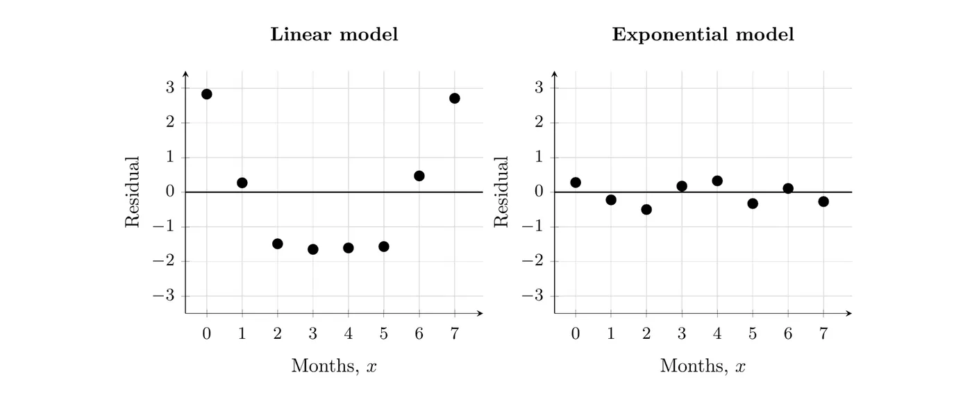
The linear model's residuals are positive at both ends and negative in the middle, a clear U shape. The data curve upward away from the line, so the linear model is not appropriate. The exponential model's residuals are small (none is more than about

0.5

from 0) and scatter above and below 0 with no pattern. The exponential model is more appropriate.

Part (c).

y = 40.02(1.120)^{12} \approx 155.9

The model predicts about 156 thousand users after 12 months. For comparison, the linear model predicts

6.86(12) + 37.47 \approx 119.8

, about 120 thousand. Predictions far outside the data are risky for any model, and that's exactly where the choice of model matters most.

Errors: Overestimates and underestimates

The error of a model at an input can be described two ways:

Signed error: the residual itself, with its sign. The sign tells you the direction: is the model too high or too low?

Absolute error: the absolute value of the residual, $|\text{actual} - \text{predicted}|$ . This only tells you the size of the miss.

Looking at the errors over an interval can show that a model consistently overestimates or underestimates there. The linear app model, for example, overestimates from month 2 through month 5 and underestimates at both ends.

The context tells you which kind of error is safer:

Water or fuel for a trip: an overestimate is safer, since you'd rather carry extra.

The weight a shelf or bridge can hold: an underestimate is safer.

Time needed to finish a project before a deadline: an overestimate is safer.

Money a business expects to earn when making a budget: an underestimate is safer.

Example 3: Water for a hike

A hiker uses the model

W(t) = 0.5t + 0.2

to predict how much water, in liters, she needs for a hike that lasts

t

hours. Here is what she actually drank on four past hikes:

$t$ (hours)	2	4	6	8
Actual water used (L)	1.1	2.0	3.2	4.5

(a) Find the residuals. (b) Where does the model overestimate, and where does it underestimate? (c) Which type of error is more dangerous here, and what should she do for an 8-hour hike?

Part (a). Find each prediction, then subtract it from the actual value.

$t$	Predicted $W(t)$	Actual	Residual
2	1.2	1.1	$-0.1$
4	2.2	2.0	$-0.2$
6	3.2	3.2	$0$
8	4.2	4.5	$0.3$

Part (b). The residuals are negative at 2 and 4 hours, so the model overestimates on short hikes. It's exact at 6 hours. The residual is positive at 8 hours, so the model underestimates on the long hike.

Part (c). Underestimating is the dangerous error, because she could run out of water on the trail. Overestimating only means carrying a little extra. The model underestimated the 8-hour hike by 0.3 L, so for long hikes she should pack more than the model says: at least 4.5 L for 8 hours instead of 4.2 L.

Notice the residuals go from negative to positive as

t

increases. That pattern means her water use grows faster than a line, so a model with an increasing rate of change might fit better.

Common mistakes

Flipping the residual. It's actual minus predicted. A positive residual means the model was too low.

Choosing a model because the graph “looks close.” Several models can look close. Check the residual plot and the context.

Accepting a curved residual plot because the residuals are small. A clear pattern means the model type is missing part of the trend.

Putting the wrong variable on the horizontal axis. A residual plot uses the input variable on the horizontal axis.

Trusting predictions far outside the data. Even the best model can fail when you extrapolate.

Back Next