2.15 - Semi-log Plots

Overview

A semi-log plot is a graph where the

y

-axis is on a logarithmic scale and the

x

-axis stays normal. Its big payoff: exponential data shows up as a straight line. That gives you a quick visual test for whether an exponential model fits, and it lets you use everything you know about lines to build that model.

What a semi-log plot is

On a normal axis, equal steps add the same amount: 0, 1, 2, 3. On a logarithmic scale with base

n

(where

n > 1

), equal steps multiply by

n

. With base 10, the gridlines are labeled 1, 10, 100, 1000, and each step up is 10 times bigger than the one before.

In a semi-log plot only one axis gets this treatment, and in AP Precalculus it's always the

y

-axis. The height of a point is really

\log y

, even though the label shows

y

itself.

Halfway between 10 and 100 is not 55. It's $10^{1.5} \approx 31.6$ , because height measures $\log y$ , and halfway between $\log 10 = 1$ and $\log 100 = 2$ is 1.5.

The smaller gridlines between 10 and 100 are 20, 30, and so on up to 90. They get closer together as you go up.

There's no 0 on a log scale (since $\log 0$ is undefined), so semi-log plots only work for positive $y$ -values.

Why exponential data looks linear

Take the log of both sides of an exponential model

y = ab^x

, then use the product and power properties from Topic 2.12:

\log_n y = \log_n\left(ab^x\right) = \log_n a + \log_n\left(b^x\right) = \log_n a + x\log_n b

That's a linear function of

x

, with slope

\log_n b

and vertical intercept

\log_n a

. A semi-log plot graphs

\log_n y

against

x

, so data or functions with exponential characteristics appear linear on a semi-log plot.

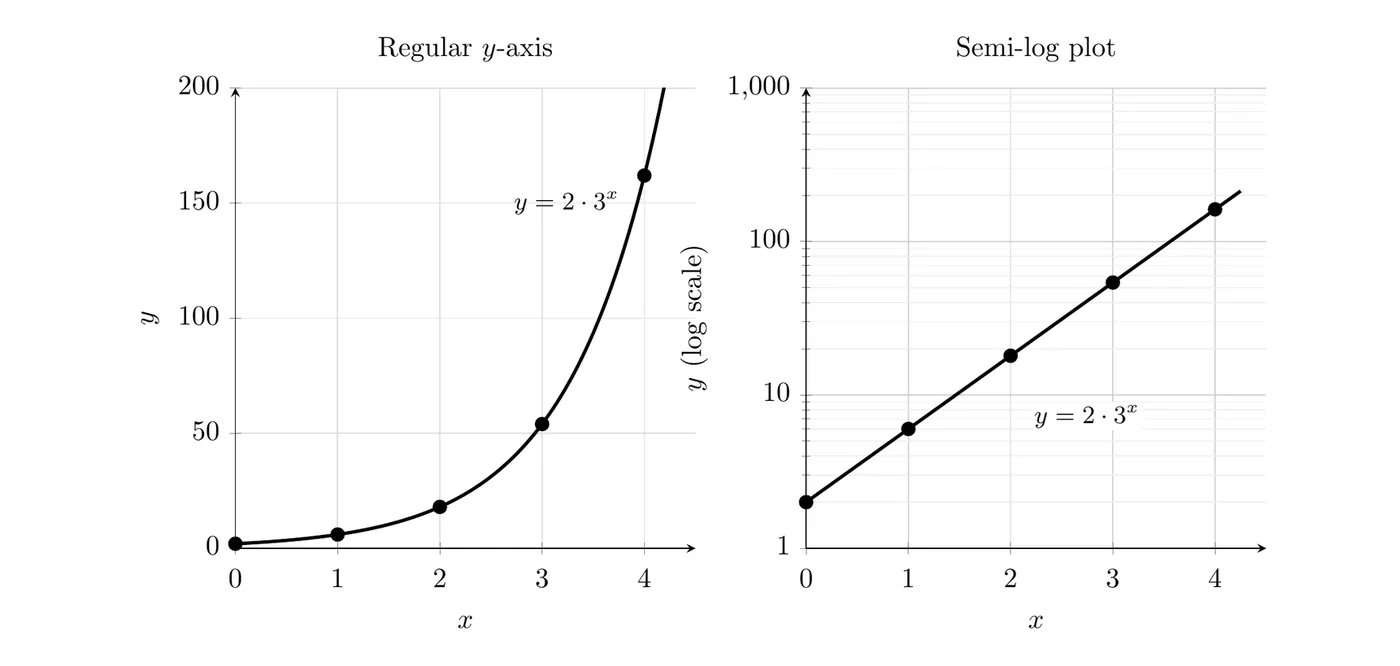
On regular axes,

y = 2 \cdot 3^x

curves up steeply. On the semi-log plot, the same points (

y = 2, 6, 18, 54, 162

) sit on a straight line. Each step of 1 in

x

multiplies

y

by 3, and multiplying by 3 always moves up the same distance on a log scale (

\log 3 \approx 0.477

Is an exponential model appropriate?

To decide, make a semi-log plot of the data (or take the log of every

y

-value) and look at the shape:

The points fall close to a line: an exponential model $y = ab^x$ is appropriate.

The points keep bending: the data isn't exponential. For example, $y = x^2$ bends on a semi-log plot, because each step of 1 in $x$ multiplies $y$ by a smaller factor each time ( $\times 4$ , then $\times 2.25$ , then about $\times 1.78$ ).

Exponentials with a constant added

Real data often looks like an exponential plus a constant,

y = ab^x + k

. On a semi-log plot that isn't a perfect line. But if the logs of the outputs trend linear for large input values, a transformation of an exponential function can model the data. When

ab^x

gets large, the constant

k

hardly matters, so the points line up.

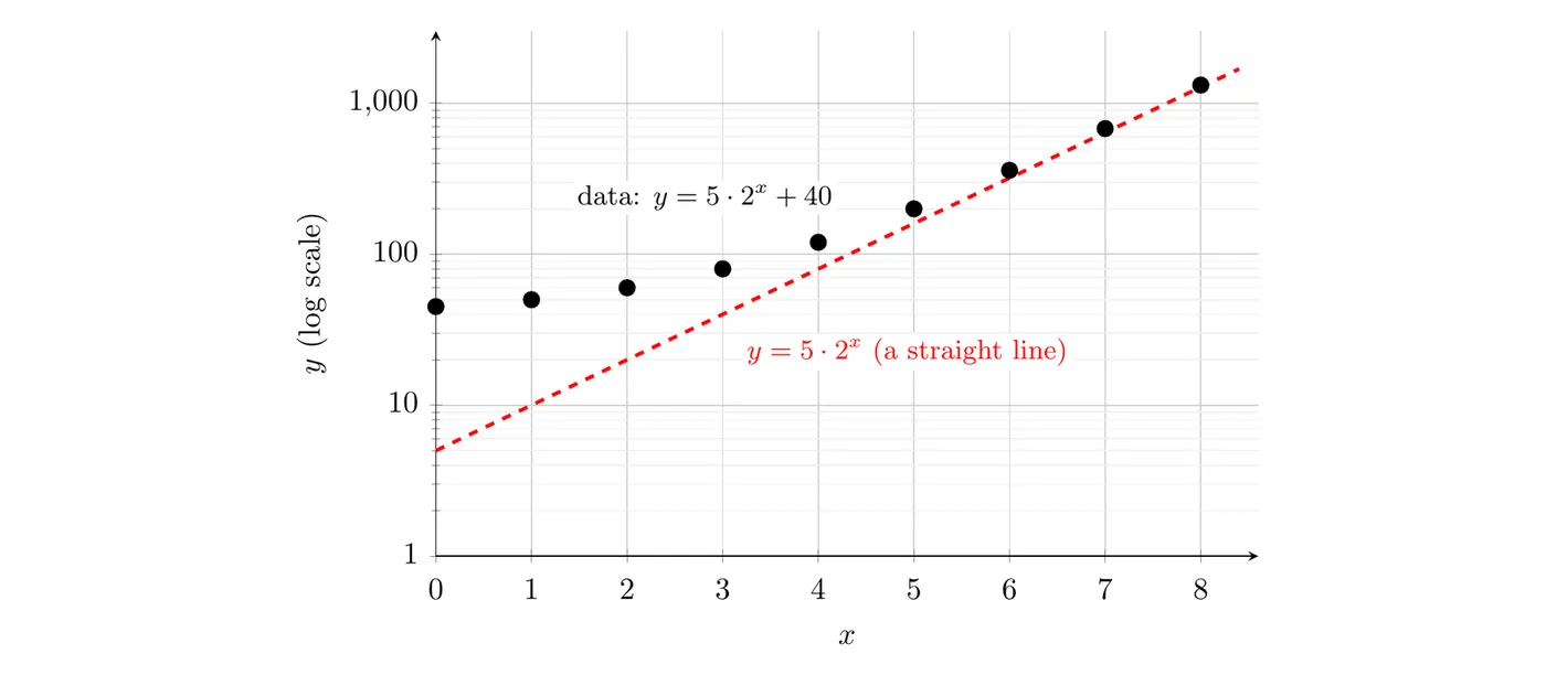
Here the data comes from

y = 5 \cdot 2^x + 40

. For small

x

, the

+40

is most of each value and the points bend. For large

x

, they line up along the line for

5 \cdot 2^x

, rising at the same steady rate. That's an advantage of semi-log plots: you don't need to figure out the constant and subtract it from every

y

-value first. The straight trend for large inputs already tells you a transformed exponential model fits.

Linearizing exponential data

Linearizing means turning exponential data into linear data by taking the log of every output. For an exponential model

y = ab^x

, the matching linear model for the semi-log plot is

\log_n y = \left(\log_n b\right)x + \log_n a

where

n > 0

and

n \neq 1

is the base of the log (usually 10 or

e

). The pieces match up like this:

Exponential model $y = ab^x$	Linear model on the semi-log plot
growth factor $b$	linear rate of change (slope) $\log_n b$
initial value $a$	initial linear value (vertical intercept) $\log_n a$

To go back from the line to the exponential, undo the logs:

b = n^{\text{slope}}

and

a = n^{\text{intercept}}

Every technique you use for linear functions works on a semi-log graph: the slope from two points, point-slope form, and linear regression.

Example 1: From an exponential model to a line

Find the linear model for the semi-log plot (base 10) of

y = 4(1.5)^x

\log y = (\log 1.5)x + \log 4 \approx 0.176x + 0.602

Answer:

\log y \approx 0.176x + 0.602

. On the semi-log plot, the line starts at a height of

\log 4 \approx 0.602

and rises 0.176 for each step of 1 in

x

Example 2: From a line back to an exponential model

A semi-log plot of a data set uses the natural log. The points fall along the line

\ln y = 0.3x + 2

. Find an exponential model for the data.

The slope is

\ln b = 0.3

, so

b = e^{0.3} \approx 1.350

. The intercept is

\ln a = 2

, so

a = e^2 \approx 7.389

y = e^{0.3x + 2} = e^2\left(e^{0.3}\right)^x \approx 7.389(1.350)^x

Answer:

y \approx 7.389(1.350)^x

Example 3: Modeling data with a semi-log plot (AP-style)

Suppose a biologist measures the area of a pond covered by an invasive water plant at the start of each week (made-up data for practice).

Weeks, $x$	0	1	2	3	4	5	6
Area covered (square meters), $y$	2.0	3.1	4.4	6.9	10.0	15.4	22.6
$\log y$	0.301	0.491	0.643	0.839	1.000	1.188	1.354

Explain why an exponential model is appropriate.

Find a linear model for $\log y$ as a function of $x$ .

Write an exponential model for $y$ .

Predict the area covered after 9 weeks.

Part 1: the values of

\log y

go up by about the same amount each week (0.190, 0.152, 0.196, 0.161, 0.188, 0.166). So the semi-log plot is close to linear, which means

y

is multiplied by about the same factor each week. That's exponential.

Part 2: run a linear regression on

(x, \log y)

. On a TI-84, put

x

in L1 and

y

in L2, set L3 = log(L2), then run LinReg(ax+b) on L1 and L3:

\log y \approx 0.1753x + 0.3050

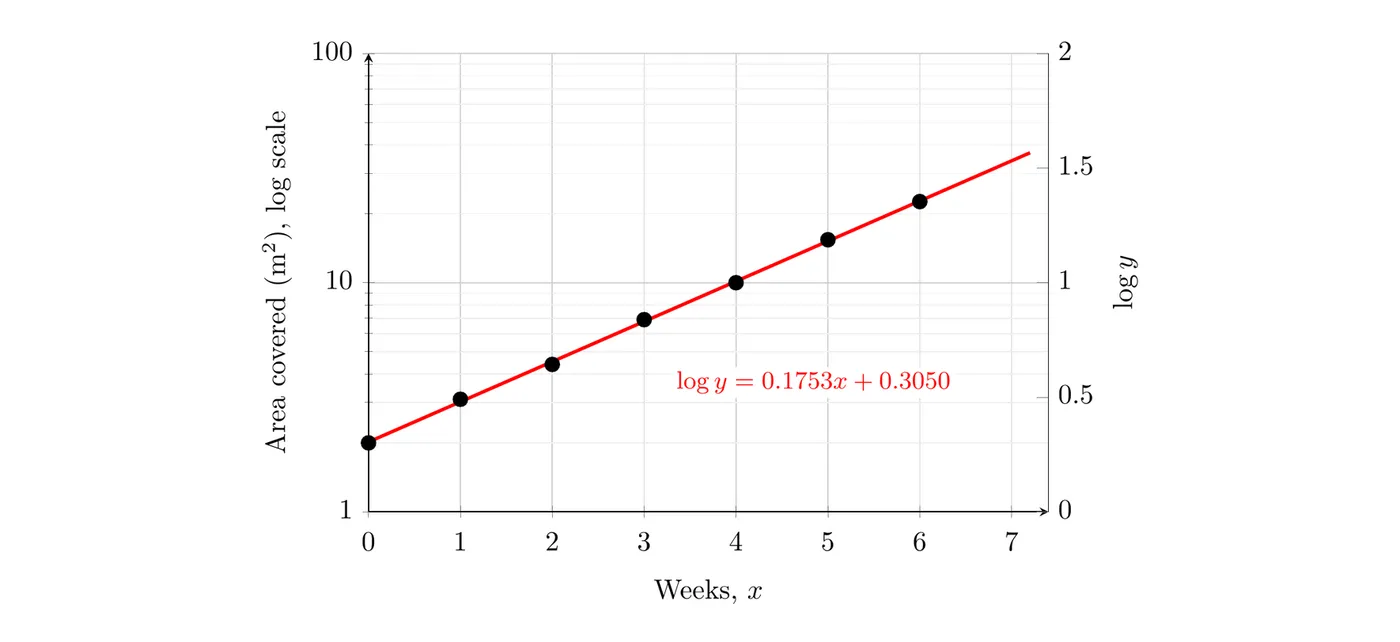
Part 3: undo the logs:

b = 10^{0.1753} \approx 1.497 \qquad a = 10^{0.3050} \approx 2.018

y \approx 2.018(1.497)^x

The calculator's ExpReg command on L1 and L2 gives the same model, because it does this linearization behind the scenes (using natural logs).

Part 4: use the linear model, then undo the log:

\log y \approx 0.1753(9) + 0.3050 = 1.8827 \quad\Rightarrow\quad y \approx 10^{1.8827} \approx 76.3

Answer: the model predicts the plant will cover about 76.3 square meters after 9 weeks, if the growth pattern continues (a real pond eventually runs out of room).

Common mistakes

Reading a log axis like a normal axis. Halfway between 10 and 100 is about 31.6, not 55.

Forgetting to undo the logs. The slope of the semi-log line is $\log_n b$ , not $b$ . The growth factor is $b = n^{\text{slope}}$ .

Mixing bases. If you linearize with $\log$ (base 10), undo with powers of 10. If you use $\ln$ , undo with powers of $e$ .

Ruling out an exponential model because of a bend at small $x$ . Look at the trend for large inputs. The data may be an exponential plus a constant.

Putting the log scale on the $x$ -axis. In this course, semi-log plots scale the $y$ -axis.

Back Next