3.10 - Constructing a Confidence Interval for the Difference Between Two Population Proportions

Overview

When you want to estimate how much two population proportions differ, the single number

\hat{p}_1 - \hat{p}_2

isn't enough, because it changes from sample to sample. A confidence interval gives a range of plausible values for the true difference

p_1 - p_2

. This topic covers choosing the procedure, checking its conditions, and calculating the interval, its standard error, and its margin of error. Interpreting the interval and using it to support a claim come next, in Topic 3.11.

The procedure and the parameters

Based on sample data, a confidence interval can estimate the difference between two population proportions. The procedure is a two-sample

z

-interval for a difference between population proportions.

The parameters must be defined in context. Name the difference in proportions, the response variable, and both populations. For example: "

p_R - p_U

, where

p_R

is the true proportion of all rural adults in the state who have a library card and

p_U

is the true proportion of all urban adults in the state who have a library card."

The order you subtract in only changes the sign of the answer, so pick one order and use it everywhere.

Conditions

A two-sample

z

-interval for

p_1 - p_2

requires three conditions:

Randomization condition: the data should be collected using two independent random samples or a randomized experiment.

10% condition: when sampling without replacement, each sample size must be at most 10% of its population size: $n_1 \leq 10\%N_1$ and $n_2 \leq 10\%N_2$ . This condition isn't needed when the data come from a randomized experiment.

Normality condition: the numbers of observed successes, $n_1\hat{p}_1$ and $n_2\hat{p}_2$ , and observed failures, $n_1(1 - \hat{p}_1)$ and $n_2(1 - \hat{p}_2)$ , are all at least 10.

Why observed counts? To build an interval we don't know

p_1

p_2

(that's the point of estimating them), so we check the counts we actually saw in each sample. Compare this with Topic 3.9, where the true proportions were known.

Calculating the interval

The point estimate for

p_1 - p_2

\hat{p}_1 - \hat{p}_2

. Like every interval in AP Statistics, the interval has the form

\text{point estimate} \pm \text{margin of error}

For the difference between two population proportions, that's

(\hat{p}_1 - \hat{p}_2) \pm z^* \sqrt{\frac{\hat{p}_1(1 - \hat{p}_1)}{n_1} + \frac{\hat{p}_2(1 - \hat{p}_2)}{n_2}}

This matches the formula sheet's general form: statistic

\pm

(critical value)(standard error of statistic).

Standard error

The standard error of the difference is

SE_{\hat{p}_1 - \hat{p}_2} = \sqrt{\frac{\hat{p}_1(1 - \hat{p}_1)}{n_1} + \frac{\hat{p}_2(1 - \hat{p}_2)}{n_2}}

It's the standard deviation from Topic 3.9 with the unknown

p_1

and

p_2

replaced by the sample proportions. It estimates how far

\hat{p}_1 - \hat{p}_2

typically is from the true difference

p_1 - p_2

Margin of error

The margin of error (MOE) is the critical value

z^*

times the standard error:

MOE = z^* \sqrt{\frac{\hat{p}_1(1 - \hat{p}_1)}{n_1} + \frac{\hat{p}_2(1 - \hat{p}_2)}{n_2}}

The critical value

z^*

comes from the confidence level, the same way as in Topic 3.3:

Confidence level	90%	95%	99%
Critical value $z^*$	$1.645$	$1.960$	$2.576$

For any other level, use invNorm. For 95% confidence, the middle 95% leaves

0.025

in each tail, so

z^* =

invNorm(0.975, 0, 1)

= 1.960

A higher confidence level means a larger

z^*

and a wider interval. Larger samples mean a smaller standard error and a narrower interval.

Example 1: Library cards (AP-style)

A state library system wants to estimate the difference between the proportions of rural and urban adults in the state who have a library card. It selects a random sample of 300 rural adults and an independent random sample of 400 urban adults. In the samples, 141 rural adults and 236 urban adults have a library card. Construct a 95% confidence interval for the difference.

State: We want to estimate

p_R - p_U

, where

p_R

is the true proportion of all rural adults in the state who have a library card and

p_U

is the true proportion of all urban adults in the state who have a library card, with 95% confidence.

Plan: Two-sample

z

-interval for

p_R - p_U

. Check the conditions:

Randomization: two independent random samples.

10%: 300 is less than 10% of all rural adults in the state, and 400 is less than 10% of all urban adults in the state.

Normality: the counts $141$ , $300 - 141 = 159$ , $236$ , and $400 - 236 = 164$ are all at least 10.

Do: The sample proportions are

\hat{p}_R = \frac{141}{300} = 0.47

and

\hat{p}_U = \frac{236}{400} = 0.59

, so the point estimate is

0.47 - 0.59 = -0.12

SE = \sqrt{\frac{0.47(0.53)}{300} + \frac{0.59(0.41)}{400}} = \sqrt{0.000830 + 0.000605} \approx 0.0379

MOE = 1.96(0.0379) \approx 0.074

-0.12 \pm 0.074 = (-0.194, -0.046)

3.10 - Constructing a Confidence Interval for the Difference Between Two Population Proportions

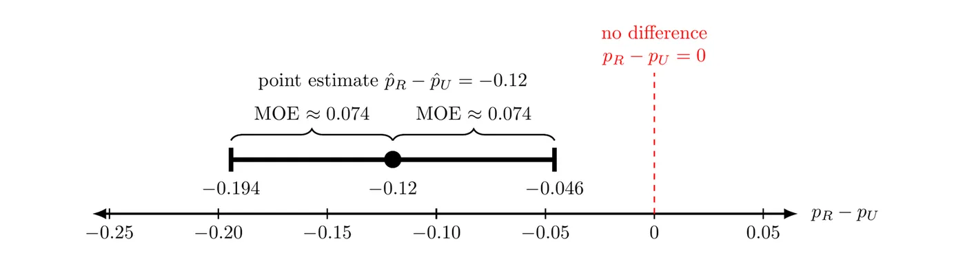
Conclude: We are 95% confident that the interval from

-0.194

-0.046

captures the true difference in the proportions of rural and urban adults in this state who have a library card (rural minus urban). Put simply, the rural proportion is plausibly between 4.6 and 19.4 percentage points lower than the urban proportion.

Calculator check: STAT, TESTS, 2-PropZInt with

x_1 = 141

n_1 = 300

x_2 = 236

n_2 = 400

, and C-Level

0.95

gives

(-0.1942, -0.0458)

If you subtract the other way (urban minus rural), the interval becomes

(0.046, 0.194)

. Same information, opposite sign.

Example 2: Reminder emails (randomized experiment)

A dental clinic wants to know whether reminder emails get more patients to book a cleaning. It recruits 360 volunteers who are overdue for a cleaning and randomly assigns 240 of them to get a reminder email and the other 120 to get no reminder. Within 30 days, 108 patients in the email group and 36 in the no-reminder group booked a cleaning. Construct a 90% confidence interval for the difference in the proportions.

State: We want to estimate

p_E - p_N

, where

p_E

is the true proportion of patients like these who would book a cleaning within 30 days if they got a reminder email and

p_N

is the true proportion who would book a cleaning within 30 days with no reminder, with 90% confidence.

Plan: Two-sample

z

-interval for

p_E - p_N

Randomization: patients were randomly assigned to the two groups (a randomized experiment).

10%: not needed, because the data come from a randomized experiment, not from sampling a population.

Normality: the counts $108$ , $240 - 108 = 132$ , $36$ , and $120 - 36 = 84$ are all at least 10.

Do:

\hat{p}_E = \frac{108}{240} = 0.45

and

\hat{p}_N = \frac{36}{120} = 0.30

, so the point estimate is

0.45 - 0.30 = 0.15

SE = \sqrt{\frac{0.45(0.55)}{240} + \frac{0.30(0.70)}{120}} = \sqrt{0.001031 + 0.001750} \approx 0.0527

The groups don't have to be the same size. Each term under the square root uses its own group's sample size.

MOE = 1.645(0.0527) \approx 0.087

0.15 \pm 0.087 = (0.063, 0.237)

Conclude: We are 90% confident that the interval from

0.063

0.237

captures the true difference in the proportions of patients like these who book a cleaning within 30 days (email minus no reminder). The volunteers weren't a random sample, so the results apply to patients like the ones in this study. Using an interval like this to back up a claim, such as "reminders work," is the focus of Topic 3.11.

Common mistakes

Defining the parameter as $\hat{p}_1 - \hat{p}_2$ . The parameter is the difference in the true population proportions, $p_1 - p_2$ , described in context.

Not saying which way you subtracted. A negative interval means nothing to a reader who doesn't know the order.

Checking normality with only one sample, or with proportions instead of counts. All four observed counts must be at least 10.

Requiring the 10% condition for an experiment, or calling volunteers a random sample.

Adding standard errors. Add the two variance terms under one square root.

Pooling the proportions. A confidence interval uses each sample's own $\hat{p}$ . A combined (pooled) proportion is only used in the test for a difference (Topics 3.12 and 3.13).

Back Next