

3.2 - Sampling Distributions for Sample Proportions
Overview
Take a random sample and compute . Take another random sample, and you'll almost surely get a different . The sampling distribution of describes that variation: its center, its spread, and its shape. Once you know those, you can find probabilities about , and that's the foundation for every interval and test in this unit.
What the sampling distribution of is
The sampling distribution of is the distribution of the values of from all possible samples of the same size from the same population. (You saw sampling distributions and simulations in Topic 2.12.)
It connects directly to the binomial distribution from Topic 2.10. If is the number of successes in the sample, then , and when the sampled values are independent, is binomial with trials and success probability .
Keep three distributions straight:
- Population distribution: the value of the variable for every individual in the population. Each one is a success or a failure, and the proportion of successes is .
- Sample data: the successes and failures in your one sample, with proportion .
- Sampling distribution: the values of from all possible samples of size .
Mean and standard deviation
For a population with proportion , when the sampled values are independent, the sampling distribution of has
Both formulas are on the AP formula sheet.
Why they work: The count is binomial, so its mean is and its standard deviation is . Dividing a random variable by divides its mean and its standard deviation by :
What the formulas tell you:
- : the sampling distribution is centered at the true proportion. That's exactly why is an unbiased estimator of (Topic 3.1).
- shrinks as grows: bigger samples give less variable estimates. Because sits under a square root, you have to multiply the sample size by 4 to cut the standard deviation in half.
Conditions
The formulas and the normal shape only hold when certain conditions are met. AP graders want each condition checked in context with numbers, not just named.
When sampling without replacement
Most real samples are taken without replacement (you don't survey the same person twice). Two conditions must be met:
- Randomization condition: the data should be collected using a random sample. Without randomness, there's no sampling distribution to describe, and the sample could be biased.
- 10% condition: the population size must be at least 10 times the sample size, , where is the population size and is the sample size. Sampling without replacement makes the draws slightly dependent (each person you pick changes who's left). When the sample is at most 10% of the population, that dependence is small enough to ignore, so the formula for is accurate.
For an approximately normal shape
The sampling distribution of is approximately normal when the sample size is large enough. To check, the expected number of successes and the expected number of failures must both be at least 10:
This is the normality condition (many teachers call it the large counts condition). Here you use , the population proportion, because in this topic is known. In Topic 3.3 you'll check the observed counts instead, because there is unknown.
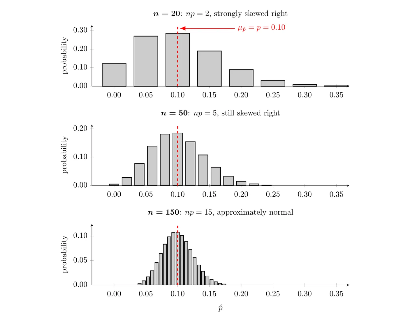
The figure shows the sampling distribution of when (from binomial probabilities) for three sample sizes. With , only successes are expected, and the distribution is strongly skewed right: can't go below 0, but it can stretch out to the right. As grows, the distribution gets narrower and more symmetric. At , and are both at least 10, and the shape is approximately normal.
Don't mix up the two kinds of conditions. The 10% condition is about independence (so the standard deviation formula is right). The normality condition is about shape (so you can use a normal distribution).
Interpreting in context
The mean, standard deviation, and probabilities for a sampling distribution of should always be interpreted in the context of the specific population. These templates work:
- Mean: "If we took many random samples of size from [population], the sample proportion who [response] would average about [value of ]."
- Standard deviation: "In random samples of size , the sample proportion of [population] who [response] typically varies by about [value of ] from the true proportion, [value of ]."
- Probability: "There's about a [probability] chance that a random sample of [individuals] gives a sample proportion of [value] or less (or more)."
Example 1: Mean and standard deviation
Suppose 62% of the 3,000 students at a community college work a part-time job. The dean's office will survey a simple random sample (SRS) of 200 students. Find and interpret the mean and standard deviation of the sampling distribution of , the proportion of sampled students who work a part-time job.
Step 1: Check the conditions for the standard deviation formula.
- Randomization: the students will be chosen with an SRS.
- 10%: , so the population is at least 10 times the sample size.
Step 2: Calculate.
Interpretation: If the dean's office took many SRSs of 200 students, the proportion who work a part-time job would average 0.62 across those samples. A typical sample proportion would be about 0.0343 (3.43 percentage points) away from 0.62.
Example 2: Finding a probability (AP-style)
In the setting of Example 1, find the probability that 55% or fewer of the sampled students work a part-time job. Would that result be surprising?
Step 1: Check the normality condition.
Both are at least 10, so the sampling distribution of is approximately normal, with mean 0.62 and standard deviation about 0.0343.
Step 2: Standardize.
Step 3: Find the area to the left.
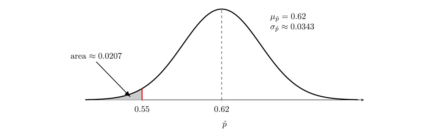
On a TI-84, use 2nd > VARS (DISTR) > normalcdf with lower bound (any very small number works), upper bound 0.55, , and . On the exam, write the distribution, its mean and standard deviation, and the boundary (as above), not just the calculator command.
Answer: About 2.1% of all SRSs of 200 students would give a sample proportion of 0.55 or less. That would be surprising, since it happens in only about 2 out of every 100 samples. If the survey did give , it would make us doubt the 62% figure. That reasoning is the core idea of significance tests, which start in Topic 3.5.
Example 3: When the normal approximation fails
A factory knows that 4% of its circuit boards have a defect. An inspector takes a random sample of 100 boards from a day's production of 5,000. Can she use a normal distribution to find ?
Step 1: Check the normality condition.
Answer: No. Only 4 defective boards are expected, so the sampling distribution of is skewed right, not approximately normal. The 10% condition is met (), but that only protects the standard deviation formula, not the shape. The difference matters: using the binomial distribution, with and is about 0.048, but a normal calculation would give about 0.021, less than half as much.
Common mistakes
- Using in when is given. In this topic the population proportion is known, so use it.
- Saying the sample is approximately normal. The sampling distribution of is approximately normal. The sample itself is just a list of successes and failures.
- Checking "n is at least 30." That rule of thumb is for means (Unit 4). For proportions, check and .
- Naming conditions without numbers. Write the actual check, like .
- Mixing up the purposes. The 10% condition protects the standard deviation formula. The normality condition protects the normal shape.
- Leaving out context. "The SD is 0.0343" earns less credit than "the proportion of sampled students who work part-time typically varies by about 0.0343 from 0.62."