3.6 - p-Values

Overview

Every hypothesis test asks the same question: if the null hypothesis were true, how surprising would our sample be? The

p

-value is the number that answers it. This topic covers what a

p

-value is, how to find one from a normal model or from a simulation, and how to interpret it in context, which the AP exam asks for often.

The null distribution

A test starts by assuming the null hypothesis

H_0

is true. Under that assumption, the test statistic has a probability distribution, called the null distribution. It shows every value the test statistic could take in repeated random samples, and how likely each one is, if

H_0

were true.

For a one-sample

z

-test for a population proportion, the test statistic is a

z

-score that measures how far the sample proportion

\hat{p}

is from the null value

p_0

(Topic 3.7 shows how to calculate it). When

H_0

is true and the conditions are met, its null distribution is approximately standard normal: centered at

0

with a standard deviation of

1

Why we need it: a sample proportion that differs from

p_0

might be nothing more than sampling variability. The null distribution tells us how much random variation to expect when

H_0

is true, so we can judge whether our result is ordinary or unusual.

What a $p$ -value is

The

p

-value is the probability of getting a test statistic as extreme as or more extreme than the one observed, assuming the null hypothesis is true. "More extreme" means farther in the direction of the alternative hypothesis.

Three parts of that definition do real work:

"Assuming $H_0$ is true": the $p$ -value comes from the null distribution, so it is calculated as if $p = p_0$ .

"As extreme or more extreme": the $p$ -value is a tail area. It is not the probability of getting exactly the value you observed.

"In the direction of $H_a$ ": the alternative hypothesis decides which tail (or tails) you use.

Which tail? Let the alternative decide

Let

x

stand for the observed value of the test statistic (a number like

1.85

). The

p

-value is:

Alternative hypothesis	$p$ -value	Area you find
$H_a\colon p > p_0$	$P(z \geq x)$	at or above $x$ (right tail)
$H_a\colon p < p_0$	$P(z \leq x)$	at or below $x$ (left tail)
$H_a\colon p \neq p_0$	$P(z \leq -\|x\|) + P(z \geq \|x\|)$	beyond $-\|x\|$ and $\|x\|$ (both tails)

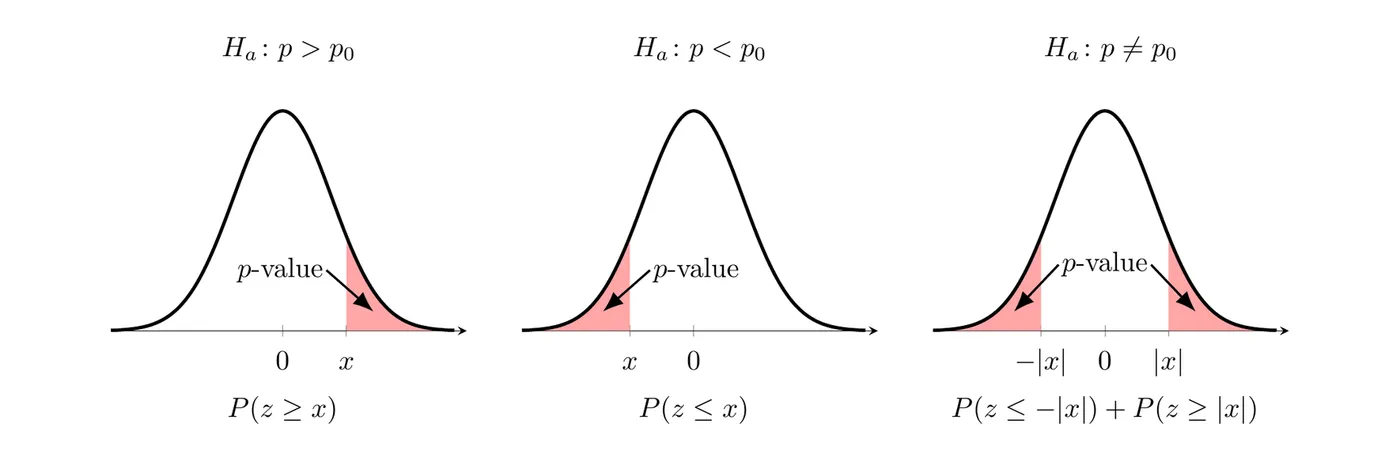
For a two-sided test, the standard normal curve is symmetric, so the two tails have equal area and the

p

-value is

2P(z \geq |x|)

Example 1: One test statistic, three $p$ -values

A test of

H_0\colon p = 0.40

gives a test statistic of

z = 1.85

. Find the

p

-value for each possible alternative.

H_a\colon p > 0.40

: shade the right tail.

P(z \geq 1.85) = 1 - 0.9678 = 0.0322

H_a\colon p < 0.40

: shade the left tail, everything at or below

1.85

P(z \leq 1.85) = 0.9678

That

p

-value is huge because the sample landed on the wrong side. The alternative says

p

is below

0.40

, but a positive

z

means the sample proportion was above

0.40

. Data on the opposite side give no evidence at all for

H_a

H_a\colon p \neq 0.40

: shade both tails.

P(z \leq -1.85) + P(z \geq 1.85) = 2(0.03216) \approx 0.0643

Answer: The same

z = 1.85

gives a

p

-value of

0.0322

0.9678

, or

0.0643

depending on the alternative. That's why you always write

H_a

before you find the

p

-value.

$p$ -values from a simulation

Sometimes there's no formula for the null distribution, or you want to see it directly. Then you simulate it: generate many samples assuming

H_0

is true, calculate the statistic for each one, and plot the results. The

p

-value is the proportion of simulated values that are as extreme as or more extreme than the observed value:

If $H_a$ uses $>$ : the proportion of simulated values at or above the observed value.

If $H_a$ uses $<$ : the proportion of simulated values at or below the observed value.

If $H_a$ uses $\neq$ : the proportion at or below $-|x|$ plus the proportion at or above $|x|$ . When the simulated statistic is $\hat{p}$ instead of $z$ , this means counting values at least as far from $p_0$ as the observed $\hat{p}$ , in either direction.

Example 2: Orange candies

A candy company says 20% of its candies are orange. Maya thinks the true proportion is higher. She buys a bag of 60 candies (assume it acts like a random sample of the company's candies) and finds 18 orange ones, so

\hat{p} = \frac{18}{60} = 0.30

Her hypotheses are

H_0\colon p = 0.20

and

H_a\colon p > 0.20

, where

p

is the true proportion of all the company's candies that are orange. To see whether

0.30

is surprising, she uses a computer to simulate 100 bags of 60 candies, assuming

p = 0.20

. Each dot is the proportion of orange candies in one simulated bag.

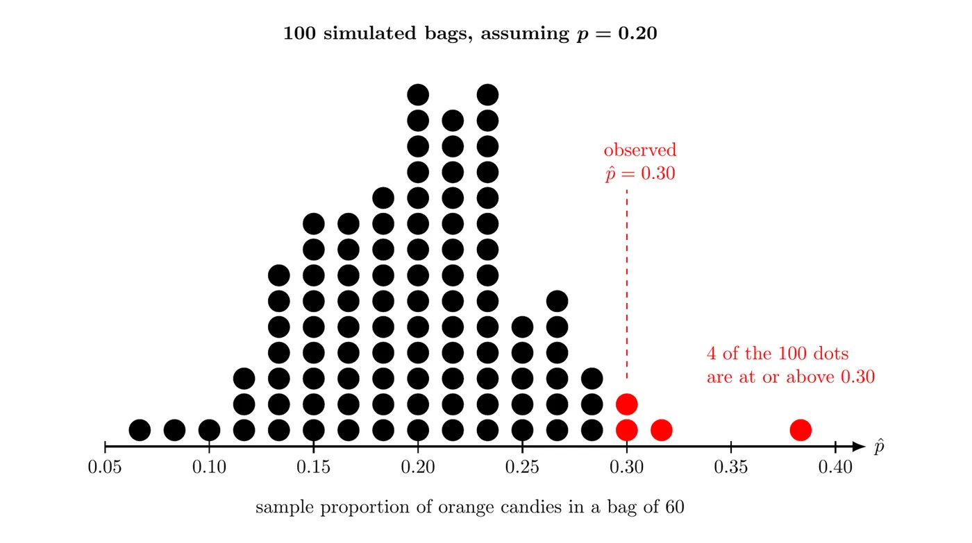
Step 1: The alternative uses

>

, so count the simulated values at or above the observed

0.30

. There are 4 of them (two at

0.30

, one at about

0.32

, and one at about

0.38

Step 2: The

p

-value is the proportion of simulated values in that tail.

p\text{-value} \approx \frac{4}{100} = 0.04

Step 3: Interpret it. Assuming the true proportion of orange candies is

0.20

, there is about a

0.04

probability of getting a sample proportion of

0.30

or higher in a bag of 60 candies just by chance.

Answer: A

p

-value of about

0.04

is small. A bag like Maya's would be unusual if only 20% of the candies were orange, so her bag gives evidence that the true proportion of orange candies is greater than

0.20

A simulation only estimates the

p

-value. The binomial probability of 18 or more orange candies in 60 is about

0.043

, and more simulated bags would land closer to it.

Two-sided version: If Maya's alternative had been

H_a\colon p \neq 0.20

, she would count simulated values at least

0.10

away from

0.20

in either direction: at or above

0.30

(4 dots) and at or below

0.10

(3 dots). The

p

-value would be about

\frac{7}{100} = 0.07

Interpreting a $p$ -value in context

An interpretation of a

p

-value must say that it was calculated assuming the null hypothesis is true, with the null value in context. On the AP exam, this is the part students most often leave out. Use this template:

Assuming the true proportion of [population and response] is [ $p_0$ ], there is a [ $p$ -value] probability of getting a sample proportion of [ $\hat{p}$ ] or [higher / lower / as far from $p_0$ ] just by chance in a random sample of [ $n$ ] [units].

"Higher" or "lower" matches the direction of

H_a

, and "as far from

p_0

" is for a two-sided test.

What small and large $p$ -values tell you

A small $p$ -value means the observed result would be unusual if $H_0$ were true. That gives evidence for the alternative hypothesis. The lower the $p$ -value, the more convincing the evidence for $H_a$ .

A $p$ -value that isn't small means the observed result would not be unusual if $H_0$ were true. That is not convincing evidence for $H_a$ . It is also not evidence that $H_0$ is true: the data are consistent with $p_0$ , but they're also consistent with plenty of other values of $p$ .

How small is small? Topic 3.7 makes this formal by comparing the

p

-value to a significance level

\alpha

chosen in advance, often

0.05

Example 3: Interpreting a $p$ -value (AP-style)

A city council member claims that more than half of the city's adults support a later start time for high schools. In a random sample of 200 adults from the city, 116 support it (

\hat{p} = 0.58

). For the test of

H_0\colon p = 0.50

versus

H_a\colon p > 0.50

, where

p

is the true proportion of all adults in the city who support a later start time, the

p

-value is

0.0118

(a) Interpret the

p

-value in context. (b) What does it tell you about the council member's claim? (c) Suppose instead that 106 of the 200 adults had supported it (

\hat{p} = 0.53

), giving a

p

-value of

0.198

. What would that tell you?

(a) Assuming the true proportion of all adults in the city who support a later start time is

0.50

, there is about a

0.0118

probability of getting a sample proportion of

0.58

or higher in a random sample of 200 adults just by chance.

(b) That's small: a result this extreme would happen in only about 1 of every 85 random samples if support were really 50%. The sample gives convincing evidence that more than half of the city's adults support a later start time, which backs the council member's claim.

(c) A

p

-value of

0.198

is not small. About 1 in 5 random samples would show 53% support or more just by chance, even if exactly half the adults supported it. So the sample would not give convincing evidence that more than half support a later start. It also would not show that exactly half support it.

Common mistakes

Calling the $p$ -value the probability that $H_0$ is true. The $p$ -value assumes $H_0$ is true. It's the probability of data like yours (or more extreme), not the probability of a hypothesis.

Leaving out "assuming $H_0$ is true." An interpretation without that condition, in context, doesn't earn credit on the AP exam.

Shading the tail where the sample landed instead of the tail $H_a$ points to. The alternative decides the direction (see Example 1).

Forgetting both tails for a two-sided test, or doubling a one-sided $p$ -value.

Treating a large $p$ -value as proof of $H_0$ . It only means the data aren't convincing evidence against $H_0$ .

Describing the probability of getting exactly $\hat{p}$ . The $p$ -value includes every result as extreme as or more extreme than the one observed.

Back Next

3.6 - p-Values

Overview

The null distribution

What a ppp-value is

Which tail? Let the alternative decide

Example 1: One test statistic, three ppp-values

ppp-values from a simulation

Example 2: Orange candies

Interpreting a ppp-value in context

What small and large ppp-values tell you

Example 3: Interpreting a ppp-value (AP-style)

Common mistakes

What a $p$ -value is

Example 1: One test statistic, three $p$ -values

$p$ -values from a simulation

Interpreting a $p$ -value in context

What small and large $p$ -values tell you

Example 3: Interpreting a $p$ -value (AP-style)