3.3 - Constructing a Confidence Interval for a Population Proportion

Overview

A single estimate like

\hat{p} = 0.58

is almost never exactly right, so statisticians attach a margin of error to it. A confidence interval gives a range of plausible values for a population proportion

p

, built from one random sample. This topic covers choosing the right procedure, checking its conditions, and calculating the interval, its standard error, and its margin of error. It also shows how to pick a sample size before you collect any data.

What a confidence interval is

A confidence interval is an interval estimate for a population parameter. Instead of one number, it gives a range:

\text{point estimate} \pm \text{margin of error}

The point estimate is the center of the interval, and the margin of error says how far the interval reaches on each side. For a single population proportion, the point estimate is

\hat{p}

, and the appropriate procedure is a one-sample

z

-interval for a population proportion. The "

z

" is there because the critical value comes from the standard normal distribution.

Defining the parameter

Before calculating anything, define the parameter in words. A complete definition names three things:

that it's the true proportion (not the sample proportion),

the response variable (what counts as a success), and

the population.

For example: "

p

= the true proportion of all adults in the state who support building a high-speed rail line." Weaker versions lose credit: "

p

= the proportion who support it" has no population, and "

p

= the proportion of the 1,000 sampled adults who support it" describes

\hat{p}

, not

p

Critical values

The critical value

z^*

is the number such that

-z^*

and

z^*

are the boundaries enclosing the middle

C\%

of the standard normal distribution.

C\%

is the confidence level. It's approximate, because the sampling distribution of

\hat{p}

is only approximately normal.

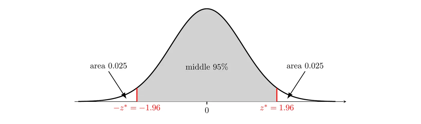
3.3 - Constructing a Confidence Interval for a Population Proportion

For 95% confidence, the middle 95% leaves 2.5% in each tail, so

z^*

is the value with 0.975 of the area to its left:

z^* \approx 1.960

. The common ones:

Confidence level	Area in each tail	$z^*$
90%	0.05	1.645
95%	0.025	1.960
98%	0.01	2.326
99%	0.005	2.576

For any other level, use invNorm on a TI-84 (2nd > VARS (DISTR) > invNorm) with area

\frac{1 + C}{2}

, writing

C

as a decimal. For 92% confidence, invNorm(0.96, 0, 1) gives

z^* \approx 1.751

Standard error

In Topic 3.2, the standard deviation of

\hat{p}

was

\sqrt{\frac{p(1 - p)}{n}}

. But when you're building an interval,

p

is exactly what you don't know. So you substitute

\hat{p}

for

p

. The result is the standard error (SE), an estimate of the standard deviation of the sampling distribution of a statistic:

SE_{\hat{p}} = \sqrt{\frac{\hat{p}(1 - \hat{p})}{n}}

The standard error measures the typical amount that

\hat{p}

varies from the true value of

p

from sample to sample.

Margin of error

The margin of error (MOE) of

\hat{p}

is the critical value times the standard error:

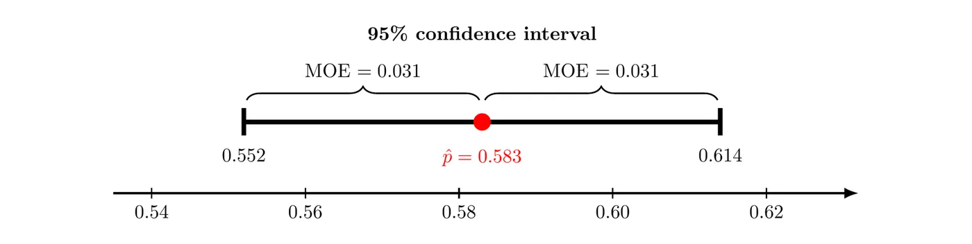
MOE = z^* \cdot SE_{\hat{p}} = z^* \sqrt{\frac{\hat{p}(1 - \hat{p})}{n}}

It's half the width of the confidence interval. So if you're given an interval

(a, b)

, you can recover both pieces:

\hat{p} = \frac{a + b}{2} \qquad MOE = \frac{b - a}{2}

The interval

Putting the pieces together, the one-sample

z

-interval for a population proportion is

\hat{p} \pm z^* \sqrt{\frac{\hat{p}(1 - \hat{p})}{n}}

This matches the general form on the AP formula sheet: statistic

\pm

(critical value)(standard error of statistic). Here's the interval from Example 1 below, with its parts labeled:

Conditions

A one-sample

z

-interval for a population proportion requires three conditions:

Randomization condition: the data should be collected using a random sample.

10% condition: when sampling without replacement, the population size must be at least 10 times the sample size, $n \le 10\%N$ , where $N$ is the population size.

Normality condition: the observed number of successes, $n\hat{p}$ , and the observed number of failures, $n(1 - \hat{p})$ , are both at least 10.

Notice that the normality condition uses

\hat{p}

here. Since

p

is unknown, you check the actual counts in your sample. Each procedure in this unit plugs in a different value:

Situation	Normality check uses	Why
Sampling distribution of $\hat{p}$ (Topic 3.2)	$p$	$p$ is known
Confidence interval for $p$ (this topic)	$\hat{p}$ , the observed counts	$p$ is unknown
Significance test for $p$ (Topic 3.5)	$p_0$ , the null value	the test assumes $H_0$ is true

The four steps

On the AP exam, a complete confidence interval answer has four steps, and every interval in Units 3 and 4 uses them:

State: the parameter, defined in context, and the confidence level.

Plan: name the procedure (here, a one-sample $z$ -interval for a population proportion) and check each condition in context.

Do: calculate the interval, showing the formula with your numbers plugged in.

Conclude: interpret the interval in context. (Topic 3.4 covers interpretations in detail.)

Example 1: Constructing the interval (AP-style)

Suppose a transportation agency surveys a random sample of 1,000 adults in a state with about 6 million adults. Of those surveyed, 583 say they support building a high-speed rail line. Construct and interpret a 95% confidence interval for the proportion of all adults in the state who support the rail line.

State: We want to estimate

p

= the true proportion of all adults in the state who support building the high-speed rail line, with 95% confidence.

Plan: One-sample

z

-interval for

p

Randomization: the adults were selected in a random sample.

10%: $1{,}000 \le 10\%(6{,}000{,}000) = 600{,}000$ .

Normality: $n\hat{p} = 583 \ge 10$ and $n(1 - \hat{p}) = 1{,}000 - 583 = 417 \ge 10$ .

Do:

\hat{p} = \frac{583}{1{,}000} = 0.583

SE_{\hat{p}} = \sqrt{\frac{0.583(0.417)}{1{,}000}} \approx 0.0156

0.583 \pm 1.960(0.0156) = 0.583 \pm 0.031 = (0.552,\ 0.614)

On a TI-84: STAT > TESTS > A: 1-PropZInt, with

x = 583

n = 1000

, and C-Level 0.95. It returns (0.55244, 0.61356).

Conclude: We are 95% confident that the interval from 0.552 to 0.614 captures the true proportion of all adults in the state who support building the high-speed rail line.

Example 2: When a condition fails

A mechanic checks a random sample of 80 cars parked in a city's garages and finds 6 with a burned-out taillight. Can she use a one-sample

z

-interval to estimate the proportion of all cars in the city's garages with a burned-out taillight?

Step 1: Check normality with the observed counts. The number of successes is

n\hat{p} = 6

, which is less than 10.

Answer: No. With only 6 successes, the sampling distribution of

\hat{p}

is likely skewed right, so a normal-based interval isn't reliable. She would need a larger sample.

Example 3: Reading an interval backward

Suppose a news report says that a 95% confidence interval for the proportion of a city's residents who use the public library is

(0.450, 0.530)

. Find the point estimate, the margin of error, and the standard error.

\hat{p} = \frac{0.450 + 0.530}{2} = 0.490 \qquad MOE = \frac{0.530 - 0.450}{2} = 0.040

SE = \frac{MOE}{z^*} = \frac{0.040}{1.960} \approx 0.0204

Answer: The sample proportion was 0.490, the margin of error is 0.040 (4 percentage points), and the standard error is about 0.0204. Going one step further, solving

\sqrt{\frac{0.49(0.51)}{n}} = 0.0204

shows the sample had about 600 people.

Choosing a sample size

Researchers often decide how precise they want an estimate to be before they collect data. Rearranging the margin of error formula for

n

gives the minimum sample size needed to achieve a given margin of error:

MOE = z^* \sqrt{\frac{\hat{p}(1 - \hat{p})}{n}} \quad \Longrightarrow \quad n = \frac{(z^*)^2\, \hat{p}(1 - \hat{p})}{(MOE)^2}

Two rules:

Always round up to the next whole number. Rounding down would leave the margin of error slightly bigger than you wanted.

If $\hat{p}$ isn't available (no past data or pilot study), use $\hat{p} = 0.5$ . That makes $\hat{p}(1 - \hat{p}) = 0.25$ , its largest possible value, so you get an upper bound: a sample size that's big enough whatever the true proportion is.

Example 4: How many people to survey?

A student government wants to estimate the proportion of students at a large university who would use a late-night shuttle, with 95% confidence and a margin of error of at most 0.03.

(a) No earlier estimate exists. How many students should they survey?

n = \frac{(1.96)^2 (0.5)(0.5)}{(0.03)^2} = \frac{0.9604}{0.0009} \approx 1{,}067.1

Round up: they need at least 1,068 students.

(b) A pilot survey suggests that about 20% of students would use the shuttle. Now how many?

n = \frac{(1.96)^2 (0.2)(0.8)}{(0.03)^2} = \frac{0.614656}{0.0009} \approx 682.95

Round up: at least 683 students. Using

\hat{p} = 0.5

in part (a) gave the most conservative (largest) answer.

Common mistakes

Checking normality with a made-up $p$ . For an interval, use the observed counts of successes and failures, $n\hat{p}$ and $n(1 - \hat{p})$ .

Writing "SRS" and nothing else. Connect each condition to the problem: "the data come from a random sample of 1,000 adults in the state."

Rounding the sample size down (or to the nearest whole number). Always round up.

Using the wrong $z^*$ . For 95% confidence it's 1.960 (area 0.975 to the left), not 1.645, which is for 90%.

Defining the parameter as the sample proportion. The interval is built from $\hat{p}$ , but it estimates $p$ , the true proportion for the whole population.

Mixing up SE and MOE. The standard error is $\sqrt{\frac{\hat{p}(1 - \hat{p})}{n}}$ . The margin of error is $z^*$ times that.

Back Next