3.13 - Carrying Out a Test for the Difference Between Two Population Proportions

Overview

Once the test is set up (Topic 3.12), you calculate the test statistic and

p

-value, compare the

p

-value to the significance level, and state a conclusion in context. This topic covers those steps for the two-sample

z

-test for the difference between two population proportions, with complete four-step write-ups like the ones the AP exam scores.

The test statistic

The test statistic measures how far the observed difference in sample proportions is from the difference claimed by

H_0

(which is 0), in standard errors:

z = \frac{(\hat{p}_1 - \hat{p}_2) - 0}{\sqrt{\hat{p}_c(1 - \hat{p}_c)}\sqrt{\dfrac{1}{n_1} + \dfrac{1}{n_2}}} \qquad \text{where} \qquad \hat{p}_c = \frac{n_1\hat{p}_1 + n_2\hat{p}_2}{n_1 + n_2}

Piece by piece:

Numerator: the observed difference, $\hat{p}_1 - \hat{p}_2$ , minus the hypothesized difference, 0.

Denominator: the standard error of $\hat{p}_1 - \hat{p}_2$ when $H_0$ is true. Since $H_0$ says $p_1 = p_2$ , both samples estimate the same proportion, so the formula uses the combined proportion $\hat{p}_c$ (total successes over total sample size). It's the "When $p_1 = p_2$ is assumed" line on the AP formula sheet.

The value of $z$ : how many standard errors the observed difference is from 0. The larger $|z|$ is, the harder the data are to explain by chance alone. A positive $z$ means $\hat{p}_1$ came out larger than $\hat{p}_2$ .

This matches the formula sheet's general form,

\frac{\text{statistic} - \text{parameter}}{\text{standard error of the statistic}}

. When

H_0

is true and the conditions are met,

z

has (approximately) a standard normal distribution,

N(0, 1)

, and that's what lets you find a

p

-value.

Finding the $p$ -value

The

p

-value is an area under the standard normal curve, found with a table or technology. Which area depends on

H_a

Alternative hypothesis	$p$ -value	Area
$H_a\colon p_1 - p_2 > 0$	$P(z \geq \text{observed } z)$	Right tail
$H_a\colon p_1 - p_2 < 0$	$P(z \leq \text{observed } z)$	Left tail
$H_a\colon p_1 - p_2 \neq 0$	$2P(z \geq \|\text{observed } z\|)$	Both tails

Normal table: the table gives the area to the left of $z$ . For a right tail, subtract it from 1. For a two-sided test, double the tail area.

The whole test at once: STAT, TESTS, 2-PropZTest. Enter $x_1$ , $n_1$ , $x_2$ , $n_2$ (the counts of successes and the sample sizes, as whole numbers), choose the direction of $H_a$ , and Calculate. It reports $z$ , the $p$ -value, $\hat{p}_1$ , $\hat{p}_2$ , and $\hat{p}$ (the combined proportion).

Just a tail area: normalcdf(lower, upper, 0, 1), with 1E99 or -1E99 for an open end.

If you use the calculator on the exam, still name the procedure in words and report

z

and the

p

-value with labels. Writing the formula with your numbers plugged in protects you: if you mistype a number, the reader can still see your method.

Interpreting the $p$ -value

The

p

-value is the probability of getting a test statistic as extreme as or more extreme than the one observed (in the direction of

H_a

), assuming

H_0

is true. For this test, "assuming

H_0

is true" means assuming the two population proportions are equal. A template:

Assuming [the true proportions are equal, in context], there is a [ $p$ -value] probability of getting a difference in sample proportions ([group 1] minus [group 2]) of [observed difference] or [more / less / more in either direction] by chance alone.

In an experiment, "by chance" means by chance in the random assignment. With random samples, it means by chance in the random sampling. A small

p

-value says the observed difference would be surprising if there were really no difference. It is not the probability that

H_0

is true.

Making the decision

A formal decision compares the

p

-value to the significance level

\alpha

out loud, with both numbers written down:

Comparison	Decision	What it means
$p$ -value $\leq \alpha$	Reject $H_0\colon p_1 - p_2 = 0$	There is convincing evidence for $H_a$ .
$p$ -value $> \alpha$	Fail to reject $H_0$	There is not convincing evidence for $H_a$ .

Use

\alpha = 0.05

if the problem doesn't give one, and say so. "The

p

-value is small, so reject" doesn't earn the point. "Because the

p

-value of 0.0031 is less than

\alpha = 0.05

, we reject

H_0

" does.

Writing the conclusion

The test's result is the statistical reasoning behind your answer to the study's question. The conclusion must:

be in context, referring to the parameters and the populations (or treatments);

be stated in terms of $H_a$ : "there is convincing evidence that [ $H_a$ in context]" or "there is not convincing evidence that [ $H_a$ in context]";

use non-definitive language: never "proves," and never "accept $H_0$ ." Failing to reject $H_0$ doesn't show the proportions are equal. It means the data aren't strong enough to show a difference.

Also mind the scope. Random samples let you generalize to the populations that were sampled. Random assignment lets you say the treatment caused the difference, for subjects like those in the study.

The four steps

Step	What to write
State	The hypotheses, with both parameters defined in context, and $\alpha$
Plan	The name of the test, and the randomization, 10%, and normality conditions checked in context
Do	The sample proportions, $\hat{p}_c$ , the test statistic, and the $p$ -value
Conclude	The $p$ -value compared to $\alpha$ , the decision, and a conclusion in context in terms of $H_a$

Example 1: Reminder emails and dental cleanings (AP-style)

A dental clinic recruited 360 volunteers who were overdue for a cleaning and randomly assigned 240 of them to get a reminder email and the other 120 to get no reminder. Within 30 days, 108 patients in the email group and 36 in the no-reminder group booked a cleaning. Do the data give convincing evidence, at

\alpha = 0.05

, that reminder emails increase the proportion of patients who book a cleaning?

State: Let

p_E

= the true proportion of patients like these who would book a cleaning within 30 days with a reminder email, and

p_N

= the true proportion who would book a cleaning within 30 days with no reminder.

H_0\colon p_E - p_N = 0 \qquad H_a\colon p_E - p_N > 0 \qquad \alpha = 0.05

Plan: Two-sample

z

-test for the difference between two population proportions. Check the conditions:

Randomization: patients were randomly assigned to the two groups.

10%: not needed, since this is a randomized experiment.

Normality: $\hat{p}_c = \frac{108 + 36}{360} = 0.40$ , and the counts $240(0.40) = 96$ , $240(0.60) = 144$ , $120(0.40) = 48$ , and $120(0.60) = 72$ are all at least 10.

Do:

\hat{p}_E = \frac{108}{240} = 0.45 \qquad \hat{p}_N = \frac{36}{120} = 0.30

z = \frac{(0.45 - 0.30) - 0}{\sqrt{0.40(0.60)}\sqrt{\dfrac{1}{240} + \dfrac{1}{120}}} = \frac{0.15}{0.0548} \approx 2.74

p\text{-value} = P(z \geq 2.74) \approx 0.0031

3.13 - Carrying Out a Test for the Difference Between Two Population Proportions

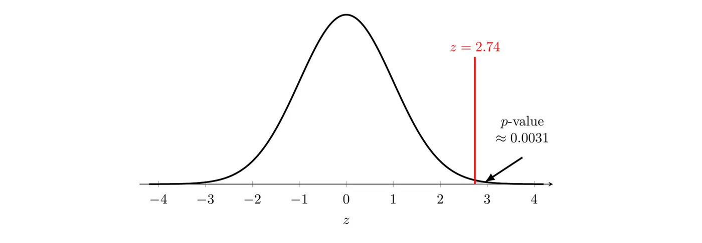
The observed difference is 2.74 standard errors above 0, and the

p

-value is the tiny shaded area to the right of

z = 2.74

Interpret the

p

-value: Assuming reminder emails make no difference (the true proportions of patients like these who book a cleaning within 30 days are equal with and without a reminder), there is about a 0.0031 probability of getting a difference in sample proportions (email minus no reminder) of 0.15 or more by chance in the random assignment.

Conclude: Because the

p

-value of 0.0031 is less than

\alpha = 0.05

, we reject

H_0

. There is convincing evidence that the true proportion of patients like these who book a cleaning within 30 days is higher with a reminder email than with no reminder. Because the reminders were randomly assigned, we can conclude the reminder emails caused the increase, for patients like the volunteers in this study.

Calculator check: 2-PropZTest with

x_1 = 108

n_1 = 240

x_2 = 36

n_2 = 120

, and

p_1 > p_2

gives

z = 2.74

and

p = 0.0031

. This agrees with Topic 3.11, where the 90% interval for

p_E - p_N

(0.063, 0.237)

, sat entirely above 0.

Example 2: Electric vehicles in two cities

A researcher took a random sample of 280 households from City A (about 180,000 households) and a separate random sample of 340 households from City B (about 240,000 households). In City A, 56 sampled households own at least one EV; in City B, 51 do. Is there convincing evidence, at

\alpha = 0.05

, that the proportion of households that own an EV differs between the two cities?

State: Let

p_A

= the true proportion of all households in City A that own at least one EV, and

p_B

= the true proportion of all households in City B that own at least one EV.

H_0\colon p_A - p_B = 0 \qquad H_a\colon p_A - p_B \neq 0 \qquad \alpha = 0.05

Plan: Two-sample

z

-test for the difference between two population proportions.

Randomization: independent random samples of households from the two cities.

10%: $280 \leq 10\%(180{,}000) = 18{,}000$ and $340 \leq 10\%(240{,}000) = 24{,}000$ .

Normality: $\hat{p}_c = \frac{107}{620} \approx 0.1726$ , so the counts are about 48.3, 231.7, 58.7, and 281.3, all at least 10.

Do:

\hat{p}_A = \frac{56}{280} = 0.20 \qquad \hat{p}_B = \frac{51}{340} = 0.15

z = \frac{(0.20 - 0.15) - 0}{\sqrt{0.1726(0.8274)}\sqrt{\dfrac{1}{280} + \dfrac{1}{340}}} = \frac{0.05}{0.0305} \approx 1.64

p\text{-value} = 2P(z \geq 1.64) \approx 0.101

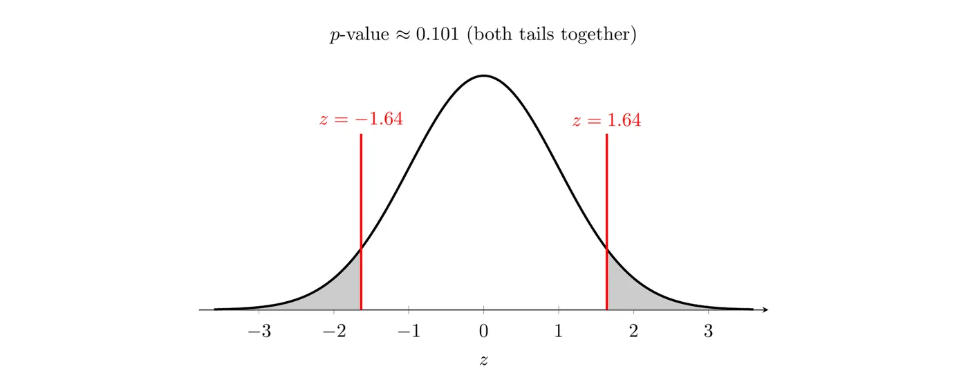
Interpret the

p

-value: Assuming the true proportions of households that own an EV are the same in City A and City B, there is about a 0.101 probability of getting a difference in sample proportions of 0.05 or more, in either direction, by chance in the random sampling.

Conclude: Because the

p

-value of 0.101 is greater than

\alpha = 0.05

, we fail to reject

H_0

. There is not convincing evidence that the proportion of all households that own an EV differs between City A and City B.

This does not show the two cities have the same proportion. A sample difference this large would happen about 10% of the time even if the cities were identical, so the data just aren't strong enough to show a difference.

Common mistakes

Mixing up standard errors: the test statistic uses $\hat{p}_c$ , the same combined proportion the calculator's 2-PropZTest uses. The separate $\hat{p}_1$ and $\hat{p}_2$ version belongs to the confidence interval.

Wrong tail: forgetting to double the tail area for a two-sided test, or doubling it for a one-sided test.

Misreading the $p$ -value: calling it the probability that $H_0$ is true, or leaving out "assuming $H_0$ is true."

A decision with no comparison: say how the $p$ -value compares to $\alpha$ , with both numbers.

Accepting $H_0$ : writing "the proportions are equal" after failing to reject.

Wrong scope: claiming cause and effect from random samples, or generalizing an experiment on volunteers to everyone.

Back Next