3.8 - Potential Errors When Performing Tests

Overview

A hypothesis test makes a decision from a sample, so it can be wrong even when every calculation is right. There are two ways to be wrong, called Type I and Type II errors. This topic covers how to describe each error in context, how to find their probabilities, what makes them more or less likely, and how to decide which one is worse. Error questions appear often on the AP exam, usually as one part of an inference free-response question.

Type I and Type II errors

Type I error: you find convincing evidence for the alternative hypothesis (because the $p$ -value is small), but $H_a$ is actually false. You rejected a null hypothesis that was true. Think "false alarm."

Type II error: you don't find convincing evidence for the alternative hypothesis (because the $p$ -value is large), but $H_a$ is actually true. You failed to reject a null hypothesis that was false. Think "missed it."

Decision	$H_0$ is actually true	$H_a$ is actually true
Reject $H_0$	Type I error	Correct decision
Fail to reject $H_0$	Correct decision	Type II error

Notice that only one error is possible after any test. If you rejected

H_0

, the only possible mistake is a Type I error. If you failed to reject, the only possible mistake is a Type II error.

Power

The power of a test is the probability that it correctly rejects a false null hypothesis. In other words, it's the chance that the test detects an effect that is really there. In the table above, power is the chance of landing in the "Correct decision" cell of the top row:

H_a

is true and the test rejects

H_0

Power depends on what the truth actually is. A test has high power for detecting a big difference from

p_0

and lower power for detecting a small one, so power is always calculated for a specific value of the parameter.

Probabilities of the errors

$P(\text{Type I error}) = \alpha$ . The significance level is defined as the probability of rejecting $H_0$ when it's true, which is exactly a Type I error. The researcher sets it to a small value, like $0.01$ , $0.05$ , or $0.10$ , before collecting data.

$P(\text{Type II error}) = 1 - \text{power}$ . If the test correctly rejects with probability equal to the power, it fails to reject (a Type II error) the rest of the time.

Ideally, the probability of a Type II error is small, so the power is large. A common goal is

P(\text{Type II error}) \leq 0.20

, which means power

\geq 0.80

Example 1: Errors in context

In Topic 3.7, a consumer group tested

H_0\colon p = 0.80

versus

H_a\colon p < 0.80

, where

p

is the true proportion of a phone company's customers who are satisfied, at

\alpha = 0.05

(a) Describe a Type I error in context and give a consequence. (b) Describe a Type II error in context and give a consequence. (c) The group rejected

H_0

. Which error could it have made?

(a) A Type I error would be finding convincing evidence that less than 80% of all the company's customers are satisfied, when really 80% are satisfied. Consequence: the group publicly criticizes an ad that was accurate.

(b) A Type II error would be not finding convincing evidence that less than 80% of all customers are satisfied, when really less than 80% are. Consequence: a misleading ad goes unchallenged, and customers choose the company based on a false claim.

(c) The group rejected

H_0

, so the only error it could have made is a Type I error.

A reliable sentence frame: "A Type I error would be finding convincing evidence that [

H_a

in context] when really [

H_0

in context]." Flip it for a Type II error.

Picturing power

Take the test from Example 1 (

n = 400

\alpha = 0.05

). It rejects

H_0

when

\hat{p}

is at or below about

0.767

, which is

z \leq -1.645

. Now suppose the true proportion of satisfied customers is really

p = 0.75

, so

H_0

is false and the right decision is to reject it.

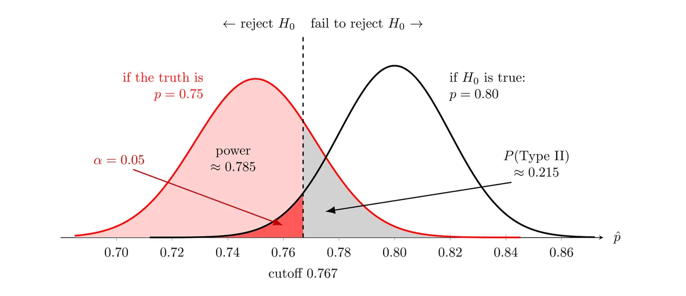
3.8 - Potential Errors When Performing Tests

The black curve is the sampling distribution of

\hat{p}

H_0

is true, and the red curve is the sampling distribution if

p = 0.75

. Everything left of the cutoff gets rejected. The dark red area under the black curve is

\alpha

, the probability of a Type I error. The light red area under the red curve is the power, about

0.785

, and the gray area under the red curve is the probability of a Type II error:

1 - 0.785 = 0.215

AP questions about power are usually conceptual: you're given the power and asked for

P(\text{Type II error}) = 1 - \text{power}

, or asked how a change to the study affects power. The picture shows why the factors below work.

What changes the power

The probability of a Type II error goes down, and the power goes up, when any one of these happens and nothing else changes:

The sample size increases. Both curves in the graph get narrower, so they overlap less.

The standard error decreases. This is the same idea in general form: less sample-to-sample variability means less overlap. For proportions, the main way to shrink the standard error is a larger sample.

The true parameter value is farther from the null value. The two curves sit farther apart, so the difference is easier to detect.

The significance level $\alpha$ increases. The cutoff moves toward the center of the null curve, so more of the true distribution lands in the rejection region. The trade-off: a larger $\alpha$ is a larger chance of a Type I error.

For the test pictured above, doubling the sample to 800 customers raises the power against

p = 0.75

from about

0.785

to about

0.960

, and raising

\alpha

0.10

raises it to about

0.870

. Raising

\alpha

trades one error for the other, but a bigger sample lowers the chance of a Type II error without raising the chance of a Type I error. That's why researchers plan their sample size before a study.

Which error is worse?

In some studies a Type I error has more serious consequences, and in others a Type II error does. The consequences of each error should be weighed before the study is run, because they shape two decisions:

The consequences of a Type I error decide $\alpha$ . Since $\alpha$ is the probability of a Type I error, a serious Type I error calls for a small $\alpha$ , like $0.01$ .

The consequences of a Type II error decide the sample size. Since sample size affects the probability of a Type II error, a serious Type II error calls for a larger sample (and possibly a larger $\alpha$ ) to get high power.

Example 2: Choosing $\alpha$ from the consequences (AP-style)

(a) A factory that makes airbag sensors accepts a defect rate of 1%. Each week, inspectors test a random sample of sensors for

H_0\colon p = 0.01

versus

H_a\colon p > 0.01

, where

p

is the true proportion of that week's sensors that are defective. If they reject

H_0

, the production line is shut down for repairs.

Type I error: shutting down the line when the defect rate is really 1%. Consequence: lost production and money.

Type II error: not finding convincing evidence of a higher defect rate when the rate really is above 1%. Consequence: faulty airbag sensors are shipped, and people could be hurt.

A Type II error is more serious here, so the factory should use a large sample and a larger significance level, like

\alpha = 0.10

, to make the power high.

(b) A drug company tests whether a new drug cures more than 60% of patients, the cure rate of the current drug:

H_0\colon p = 0.60

versus

H_a\colon p > 0.60

. If it finds convincing evidence, doctors will switch to the new drug, which costs far more and has more side effects.

Type I error: concluding the new drug cures more than 60% of patients when it doesn't. Consequence: patients switch to a more expensive drug with more side effects for no benefit.

Type II error: missing a new drug that really does cure more than 60%. Consequence: patients keep using the current drug, which still works for 60% of them.

A Type I error is more serious here, so the company should use a small significance level, like

\alpha = 0.01

Common mistakes

Describing an error without context. "Rejecting $H_0$ when it's true" isn't enough on the AP exam. Say what that means in the problem's words.

Naming an error that can't have happened. After rejecting $H_0$ , only a Type I error is possible; after failing to reject, only a Type II error is possible.

Calling $\alpha$ the probability that $H_0$ is true, or the probability of making any error. It's the probability of rejecting $H_0$ given that $H_0$ is true.

Thinking a larger sample lowers the chance of a Type I error. That chance is $\alpha$ , which the researcher sets. A larger sample lowers the chance of a Type II error.

Saying a larger $\alpha$ is always better because power goes up. It also raises the chance of a Type I error.

Forgetting that power depends on the true value of the parameter. A power value always goes with a specific alternative value, like $p = 0.75$ .

Back Next

3.8 - Potential Errors When Performing Tests

Overview

Type I and Type II errors

Power

Probabilities of the errors

Example 1: Errors in context

Picturing power

What changes the power

Which error is worse?

Example 2: Choosing α\alphaα from the consequences (AP-style)

Common mistakes

Example 2: Choosing $\alpha$ from the consequences (AP-style)